Fault identification of the vehicle suspension system based on binocular vision and kinematic decoupling

Suspension faults have a detrimental impact on the safety and handling stability of a vehicle. Therefore, monitoring the condition of suspension systems is significant to ensuring the safe operation of modern vehicles. This paper proposes an online monitoring scheme that utilizes binocular vision and kinematic decoupling, to fulfill real-time monitoring requirements for suspensions. To implement the proposed method, a system consisting of a binocular camera and an inertial measurement unit (IMU) is established for acquiring vibration signals from the vehicle body. Additionally, the vibration signals are analyzed with stochastic subspace identification (SSI) method to determine the modal parameters of suspensions. By analyzing the changes in suspension modal parameters, the types and degrees of faults in the suspension system were identified and evaluated. The experimental results show that the proposed method can effectively extract the vertical vibration signals of a vehicle. Moreover, the fault identification method based on modal parameters can identify the changes in vehicle modal parameters with high reliability under different spring stiffness, damper damping and tire pressure conditions. The proposed method is proven to be effective in identifying suspension faults, paving a way for online condition monitoring and fault diagnosis of vehicle suspensions.

1 Introduction

Over the years, automobiles have become an essential part of our lives (Abubakar et al., 2021). With the rapid development of the automobile industry, the safety, reliability and comfort of automobiles have been given much importance (Luo et al., 2019). As one of the most critical load bearing components of vehicles, automotive suspension plays a significant role in ensuring the vehicle's safety, smoothness and handling stability (Jeong et al., 2020). However, the long-term operation of a vehicle will probably lead to different faults in suspension components. Eventually, the suspension will not perform properly. The potential faults would cause enormous human casualties and economic losses (Alcantara et al., 2016). Therefore, it is necessary to monitor the suspension system for early faults, which could prevent further damage.

In the past decade, condition monitoring and fault diagnosis methods for suspension systems have become a significant research subject (Sai et al., 2023). Under tough driving conditions, the internal components of the suspension would break down. Some typical component faults include spring faults, damper faults, and tire pressure faults. Based on different detection techniques and analysis methods, researchers have conducted several studies on the three types of typical suspension system faults mentioned above. For spring faults, Wang and Yin (2014) proposed a clustering-based method. Accelerator sensors are installed at the four corners of the vehicle body to acquire acceleration data. The Fisher discriminant analysis is then applied to detect the suspension spring faults. Simulation and experiment results proved that the clustering-based method was efficient in detecting and isolating spring faults of different degrees. Wei et al. (2012) applied the Kalman filter to spring faults in a railroad vehicle, and the measurement signals were also collected by accelerator sensors placed on the four corners of a vehicle. The research results indicated that suspension spring failures can be detected based on residuals. In addition, Li et al. (2018, b) introduced fault indicators (FIs) into the diagnosis of bolster spring failures in heavy-haul wagons. Vibration data are acquired by the accelerator sensors installed on the left front and right rear of the train. Their findings show that the FIs are capable of detecting faults in the support springs with high sensitivity. For damper faults, Białkowski and Krężel (2017) evaluated the effect of fast Fourier transform (FFT) and cross-spectrum on damper damping loss through vibration signals acquired by accelerator pedal sensors. The findings confirmed that cross-spectrum analysis is better for damper fault identification. Dumitriu (2019) proposed a method for fault detection in dampers in railway vehicle suspension based on cross-correlation analysis of bogie accelerations. Numerical simulations and experimental results show that the fault in a damper can be detected by the decrease in the cross-correlation coefficient of the bogie accelerations. Hamed et al. (2020) studied the performance of frequency response functions (FRFs) to monitor damper damping faults. The monitoring reliability of FRFs has been demonstrated. Sorribes-Palmer et al. (2020) proposed a method for fault detection and isolation of bogie suspension components based on on-board acoustic sensors. The results show that suspension fault classification can be performed using the normalized Gini coefficient. For tire pressure faults, two detection methods exist: the direct method and the indirect method. The direct method uses pressure sensors (Velupillai and Guvenc, 2007; Zhang et al., 2009, and Wei et al., 2021) mounted on the rim of each tire to measure tire pressure directly. This method can accurately measure the inflation pressure of each tire, but it is cumbersome and costly to maintain. The indirect method reflects the tire pressure conditions by measuring and analyzing variables such as wheel vibration acceleration (Pardeshi et al., 2022; Jatakar et al., 2023), tire stiffness (Carlson and Gerdes, 2005; Han et al., 2008), effective radius (Mayer, 1994) and resonance frequency (Zhao et al., 2023). This method offers the advantages of a simple structure and low cost.

From the above studies in the literature, it can be seen that most of the research that has been carried out uses vibration sensors to monitor the condition of specific suspension components and identify faults. Vibration-sensor-based methods have been proven to be highly effective in identifying and monitoring suspension faults. However, installing specialized sensors for data acquisition would destroy the original structure and make the wiring complicated. It increases the cost of fault diagnosis. Furthermore, the measured vibration data are susceptible to interference from component vibration and complex transmission paths. In recent years, with the development of low-cost high-quality imaging equipment and significant advances in computer vision (CV) technology, vision-based vibration measurement techniques have been receiving increasing attention (Dong and Catbas, 2021). Vision-based vibration measurement technology is characterized by non-contact full-field measurement and visual analysis. It is currently most widely applied in the field of civil engineering structures (Hu et al., 2023; Liu et al., 2023; Jalendra et al., 2023; Tan et al., 2023; Shao et al., 2023, and Bai et al., 2023). In the field of mechanical structure vibration measurement, Tang et al. (2016) first employed machine vision technology in the measurement of disk vibration displacement. This method has been proven to be featured with easy operation, simple instruments, low cost and high accuracy and can effectively detect the disk vibration signals. A single high-speed-camera pseudo-stereo system with a four-mirror adapter was studied by Durand-Texte et al. (2019). The system is used to measure sub-millimeter displacements of a flat plate. The measurement results were compared with those obtained using an accelerometer and a laser vibrometer method. The results indicated that this method can detect plate displacements with a less measurement error. Spytek et al. (2023) measured the vibration of an air compressor using a novel method based on visual data. The mean frequency map was confirmed to perform excellently in structural vibration measurements. Yang et al. (2020) investigated a computer vision method for modal analysis. The research results indicate that the method is more efficient, autonomous and accurate. The research mentioned above has shown that accurate measurement of vibration can be achieved based on vision. However, most of the present vision-based vibration measurement technologies are applied to monitor the occurrence of events outside the camera carrier. Meanwhile, the camera and the measured object maintain a non-contact relationship. However, in the field of contact measurements, and especially in the area of vibration measurements of the camera carrier itself, few studies have been carried out.

Due to the complex characteristics of vehicle kinematics, there are currently no on-board camera-based vision measurement techniques for measuring a vehicle's own posture and vibration. If the posture and vibration of a vehicle can be detected by an on-board binocular camera, it is possible to realize a real-time condition monitoring and fault diagnosis technique for vehicle suspension systems. However, there are two technical difficulties with the above technique. Firstly, both translational and rotational motions happen as the camera moves with a vehicle. It is not feasible to distinguish between these two motion types solely by image analysis techniques. It is necessary to decouple the camera carrier's motion so that its translational and rotational motions can be solved. Secondly, the acquired raw data are normally quite large, complex and disorganized. How to accurately and efficiently extract the suspension fault information from the data is a challenge which needs to be addressed urgently. Therefore, a data processing algorithm with excellent real-time performance and high reliability is required.

Currently, there are two main types of widely used suspension fault diagnosis algorithms: data-driven methods and model-based methods. Data-driven methods can achieve representation learning from historical sensory data without expert knowledge. They have the ability to perform system fault diagnosis based solely on response data (Luo et al., 2018). In addition to the traditional algorithms, the principal component analysis (PCA) (Gertler and Cao, 2004; Choqueuse et al., 2012) and partial least-squares (PLS) regression (Muradore and Fiorini, 2012), a number of novel methods have been employed in fault diagnosis of different systems. Arun Balaji and Sugumaran (2021) proposed an approach based on a Bayes classifier, and two Bayes classifiers (naive Bayes and Bayesian network classifiers) were investigated for their performance in classifying automotive suspension faults. The results show that the Bayesian network classifier has the highest classification accuracy and can effectively identify faulty suspension states. Luo et al. (2018) and Huet al. (2021) investigated the application of the long short-term memory (LSTM) network method in the fault identification of automotive suspension components. It is proven that the LSTM method is highly accurate and exhibits better fault diagnosis performance. Yang et al. (2023) proposed a method to improve fault diagnosis accuracy by injecting noise. It was demonstrated that the injection of noise can improve the fault diagnosis accuracy. The strengths of the data-driven methods are obvious. However, the detection data on which the method relies are susceptible to interference from noise and various other factors, which would lead to biased results. Because of the complex operating conditions of vehicles, diverse roadway excitations and strong noise, data-driven methods are not suitable for fault diagnosis of vehicle suspensions. In contrast to data-driven methods, model-based methods rely heavily on the fundamental physical knowledge of dynamic processes. These methods can dive deeper into the nature of the dynamical systems to explain the root causes of faults as well as have better robustness and generalization capabilities (Li et al., 2020). In recent years, the stochastic subspace identification (SSI) method has been receiving increasing attention in the field of suspension fault diagnosis. It has the advantages of high immunity to interference, high accuracy, as well as the ability to perform modal identification based solely on response data. An average correlation signal-based SSI (ACS-SSI) method was presented by Chen et al. (2015a, b) in order to identify the dynamic characteristics of the chassis frame in a heavy truck. The results indicated that ACS-SSI performed excellently in identifying modal parameters of the system undergoing testing. Similarly, Liu et al. (2018) also employed the ACS-SSI method to identify dump truck suspension faults. Numerical simulations and real-vehicle tests demonstrate that it is practical to identify suspension faults through the changes in the modal energy difference (MED). In addition, Liu et al. (2019, 2020) proposed a correlation signal subset-based stochastic subspace identification to identify railway vehicle suspension faults. It proved that spring stiffness faults in suspension systems can be accurately identified based on the change in the pitch mode.

To address the described technical difficulties, this paper proposes a vibration measurement method based on binocular vision and camera carrier kinematic decoupling. The acquired vibration data were analyzed with the ACS-SSI algorithm. It effectively achieves the identification and monitoring of typical suspension faults. Firstly, a binocular camera is installed on the top of the vehicle body to collect the changes in reference markers in the image sequence during operation. Concurrently, the posture response of a vehicle caused by random road excitation is recorded. The body angle changes are captured using an inertial measurement unit (IMU). Based on these two measurement signals, decoupling calculations are performed to obtain the vertical vibration information on the vehicle body. Moreover, the vehicle suspension's modal features are identified and analyzed based on the ACS-SSI method. The effects of different suspension fault types on the vehicle's modal parameters are obtained. Eventually, the feasibility of the proposed method is verified by real-vehicle road tests.

The rest of this paper is organized as follows. Section 2 describes the technical path of this paper and elaborates the research methodology of this paper, including the principle of binocular vision and the kinematic decoupling algorithm. The results of the modal simulation analysis are presented in Sect. 3. The real-vehicle tests are conducted in Sect. 4, and the conclusions are presented in Sect. 5.

2 Background and methodology

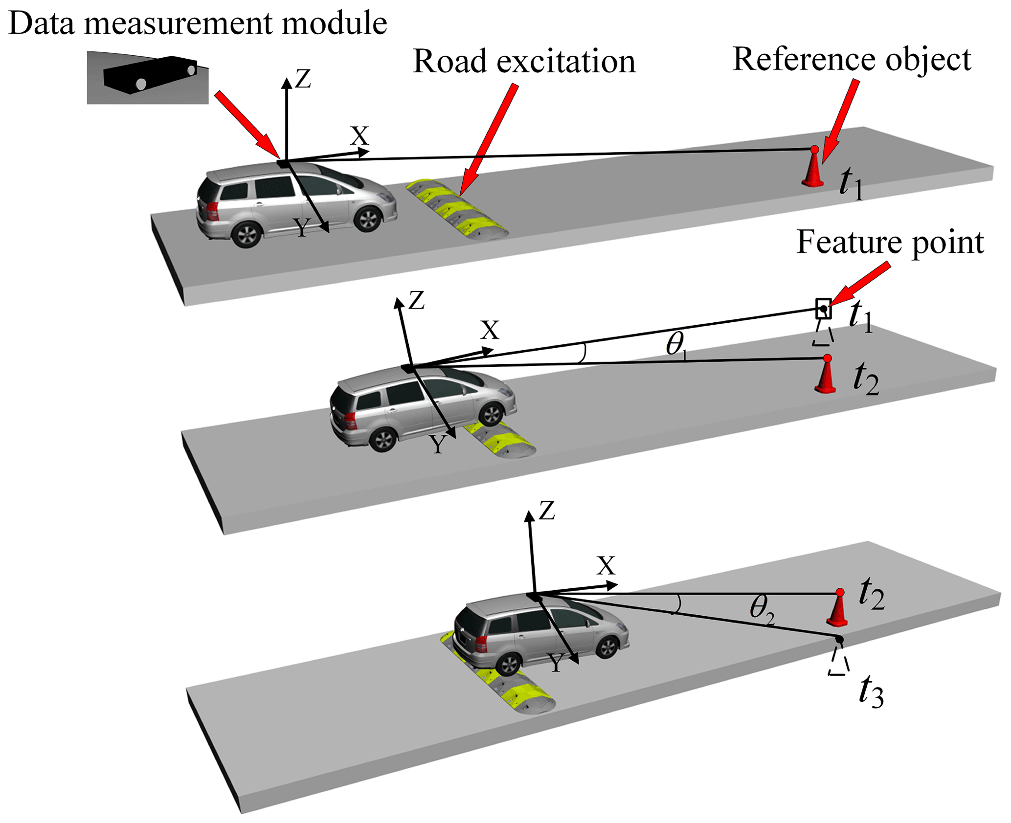
As illustrated in Fig. 1, when the vehicle is driving normally on a straight road (at moment t₁), computer vision and image processing techniques enable the binocular camera installed on the top of the body to recognize the 3D coordinates of the feature point on the reference object. This allows for the inference of the body posture based on the correspondence between the binocular camera and the 3D coordinates of the feature point, thus obtaining the spatial posture information of the vehicle body. When the vehicle is affected by road unevenness (e.g., passing a speed bump), the posture of the vehicle generates both a bounce and a pitch response with respect to the absolute coordinate system. For instance, compared with moment t₁, as the front wheels of the vehicle pass over the speed bump (at moment t₂), the feature point on the reference object produces a deflection of angle θ₁ in the camera field of view. Similarly, when the rear wheels of the vehicle cross the speed bump (at moment t₃), a deflection angle θ₂ is also generated in the camera field of view. It should be noted that it is difficult to distinguish between the type of body motions using only a binocular camera since the offset of feature points may be caused by pitch, bounce, or a combination of the two. For this reason, a device capable of measuring the body pitch angle, the inertial measurement unit (IMU), was added to the measurement system. By kinematic decoupling of the posture information and measuring the pitch angle, the vertical vibration information of the body can finally be acquired.

Figure 1 Vehicle motion generated by road excitation.

The modal parameters of the vehicle system can be identified by the ACS-SSI method from the acquired vertical vibration signals. When a suspension component fails to function, its corresponding modal parameters will change to certain degree (Chen et al., 2015a, b). Therefore, by establishing a mapping between faults and modal parameter variations, the identification of the type and degree of suspension faults can be realized (Liu et al., 2018).

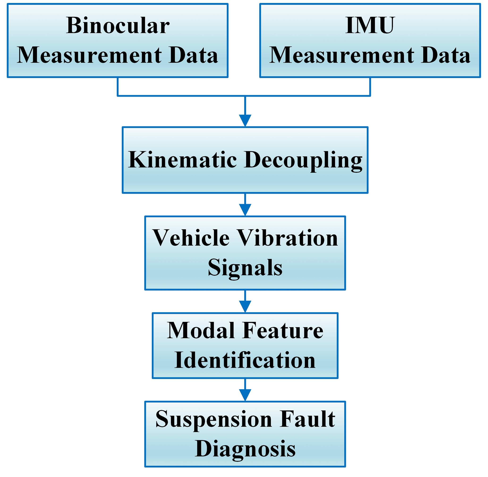
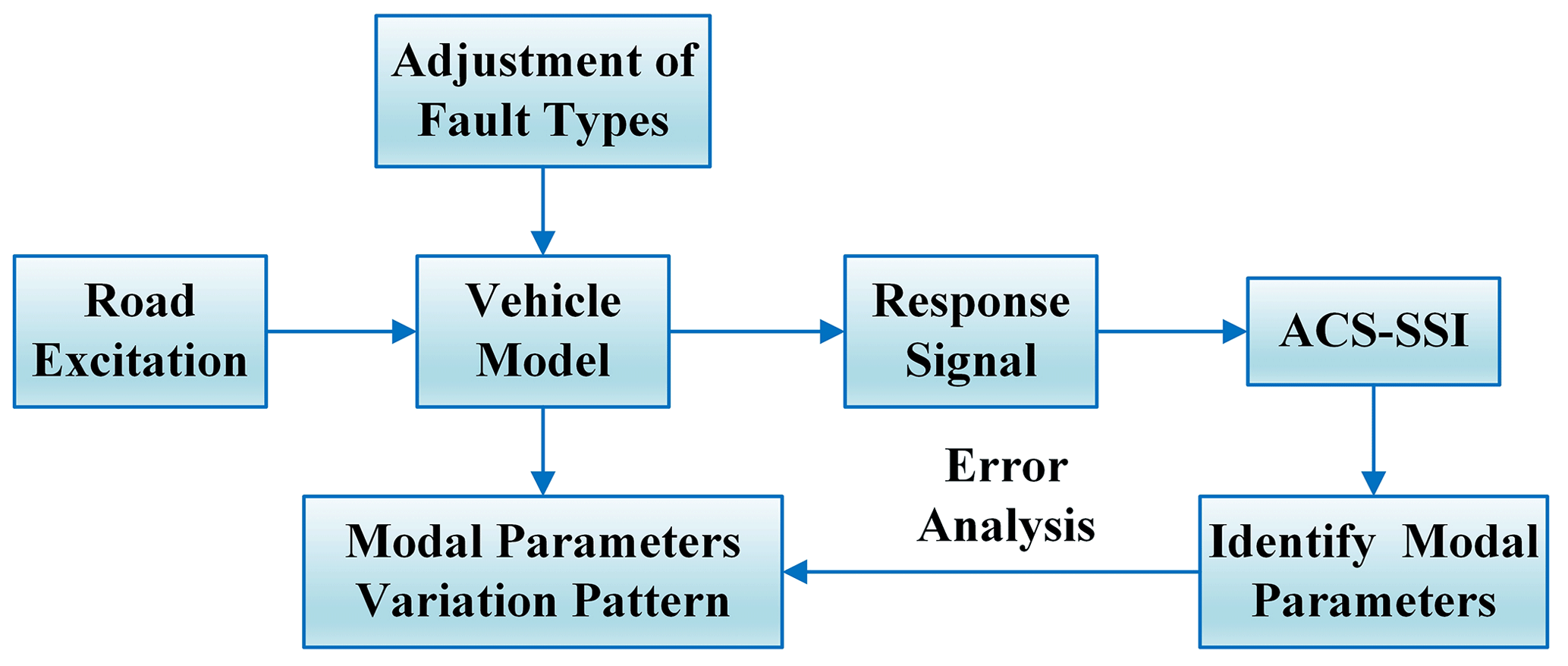
Figure 2 illustrates the process of fault identification for the vehicle suspension system. The data acquisition equipment used in the tests consisted of a binocular camera and an IMU, both of which operated synchronously during the tests. Initially, image feature recognition methods are applied to the image sequence of reference markers acquired by the binocular camera. Concurrently, the IMU is synchronized with the binocular camera to determine the body pitch angle. Subsequently, the two types of data are decoupled to obtain the vertical vibration information of the practical vehicle. In order to ensure the effectiveness of the algorithm, the body vibration information obtained from real-vehicle tests and simulations is analyzed. Finally, by adopting SSI to identify the modal parameters of the practical body vibration response, the characteristic information of the whole vehicle dynamics model can be obtained. Moreover, the fault identification of the vehicle suspension system is realized by comparing the changes in modal parameters under the influence of different faults.

Figure 2 Flowchart of suspension system fault identification.

2.1 Binocular vision system model

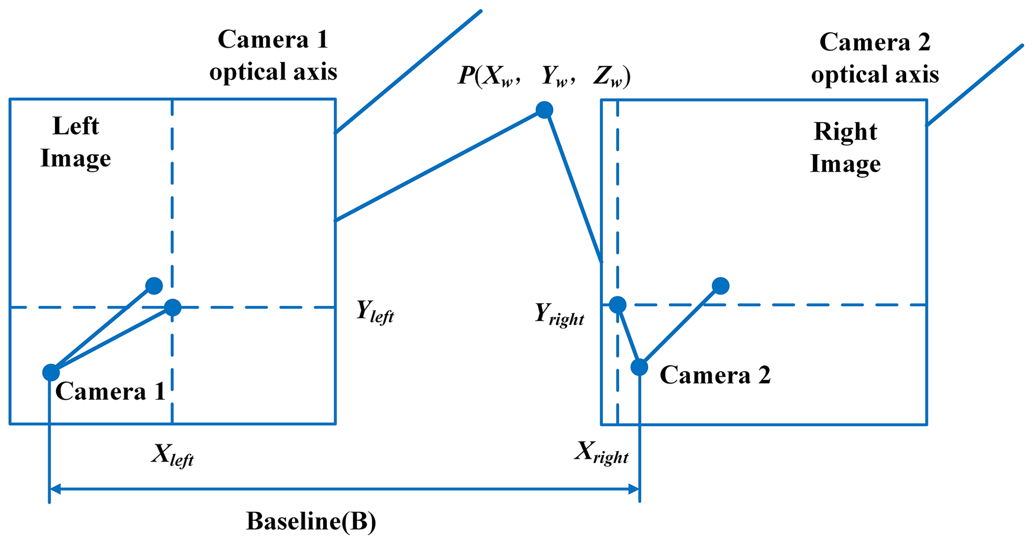
The binocular vision system usually consists of two cameras of the same specification, the same focal length, the same aperture and the same sensor area of the camera (Sun et al., 2019). Ideally, the left and right cameras are parallel to each other and remain in the same plane; the imaging model is shown in Fig. 3. In the figure, the distance between the two cameras is B. Feature point $P\left(X_{\mathrm{w}},Y_{\mathrm{w}},Z_{\mathrm{w}}\right)$ in the imaging images of the left and right cameras are $P_{\mathrm{left}}=\left(X_{\mathrm{left}},Y_{\mathrm{left}}\right)$ and $P_{\mathrm{right}}=\left(X_{\mathrm{right}},Y_{\mathrm{right}}\right)$. Since the images of the two cameras are on the same plane, the coordinate Y of the feature point P in the image coordinate system must be the same – that is, $Y_{\mathrm{left}}=Y_{\mathrm{right}}=Y$. According to the triangular geometric relationship, the following relationship can be obtained:

$$\begin{array}{}\text{(1)}& \left\{\begin{array}{lcl}{X}_{\mathrm{left}}& =& f\frac{X_{\mathrm{w}}}{Z_{\mathrm{w}}},\\ X_{\mathrm{right}}& =& f\frac{\left(X_{\mathrm{w}}-B\right)}{Z_{\mathrm{w}}},\\ Y_{\mathrm{left}}& =& Y_{\mathrm{right}}=f\frac{Y_{\mathrm{w}}}{Z_{\mathrm{w}}}.\end{array}\right.\end{array}$$

In Eq. (1), f is the camera focal length and parallax $d=X_{\mathrm{left}}-X_{\mathrm{right}}$. From this, it is clear that the 3D coordinates of the feature point $P\left(X_{\mathrm{w}},Y_{\mathrm{w}},Z_{\mathrm{w}}\right)$ in the world coordinate system can be calculated as follows:

$$\begin{array}{}\text{(2)}& \left\{\begin{array}{lcl}{X}_{\mathrm{w}}& =& \frac{B\cdot X_{\mathrm{left}}}{d},\\ Y_{\mathrm{w}}& =& \frac{B\cdot Y_{\mathrm{left}}}{d},\\ Z_{\mathrm{w}}& =& \frac{B\cdot f}{d}.\end{array}\right.\end{array}$$

From Eqs. (1) and (2), after obtaining the internal parameters of the binocular camera, baseline distance B and parallax d, the 3D coordinates of space point P can be calculated individually. However, it should be noted that if the position and posture of the camera change, the corresponding imaging plane will also undergo a projection transformation with the camera optical axis. Meanwhile, the 3D coordinates of the space point will change in this projection plane.

Figure 3 Binocular vision system model.

2.2 Principle of vehicle vibration measurement

2.2.1 Image feature point extraction

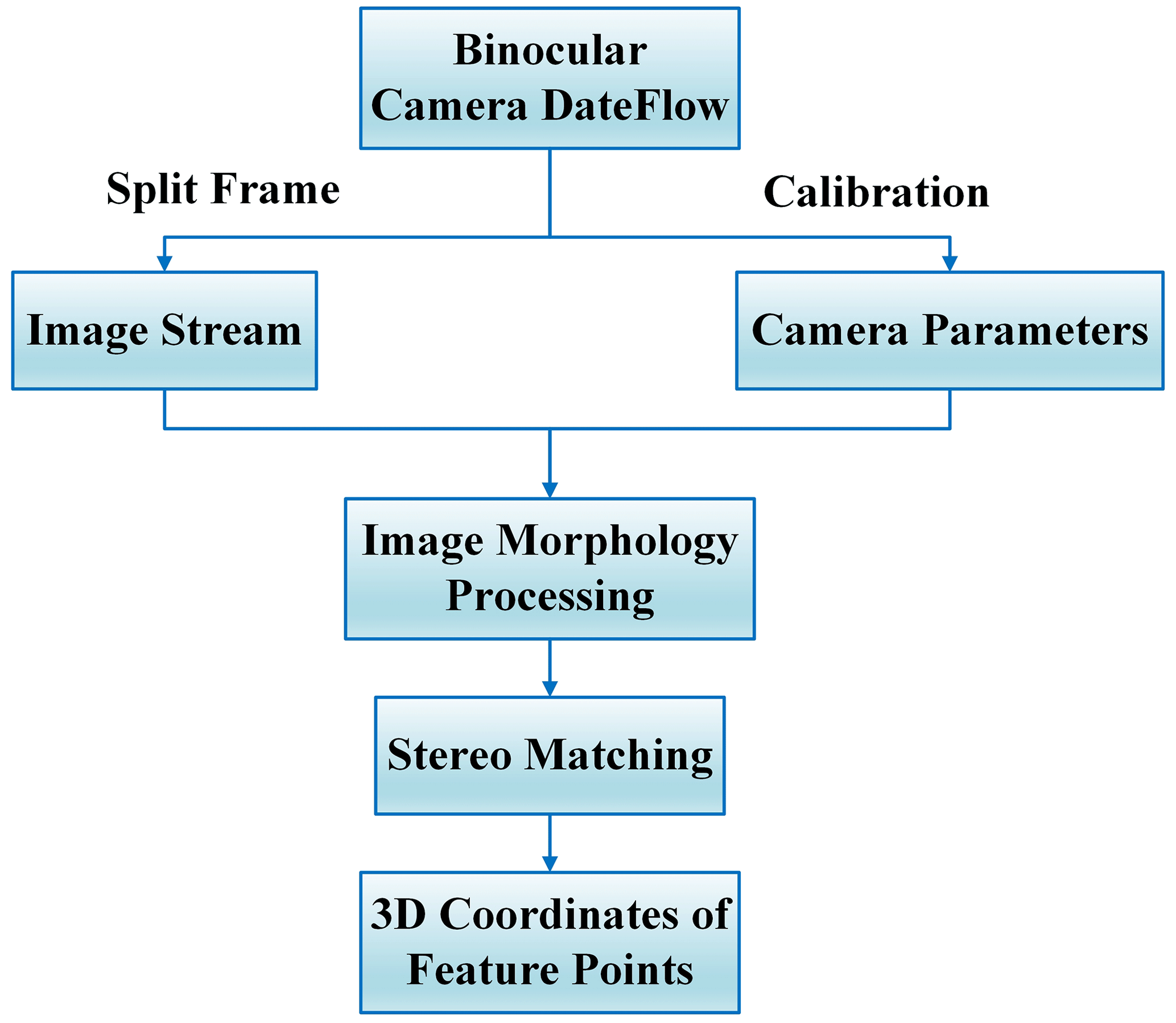
With the binocular vision technique, image feature information can be effectively extracted. Figure 4 illustrates the process of image feature point extraction. Initially, the internal and external parameters as well as the distortion coefficients of the binocular camera are used for stereo correction and stereo matching of the images. The process continues by splitting video frames to generate sequence images and applying binocular stereo matching algorithm to obtain a parallax map. Consequently, the 3D coordinates information of each pixel point of images can be obtained. Additionally, the left camera undergoes image morphology processing to calculate the pixel-connected domain in the image. By calculating the image connectivity domain properties, it can obtain the pixel coordinates of the reference markers. Eventually, the 3D coordinate information on the reference markers is obtained by searching the parallax map at the corresponding pixel coordinates.

Figure 4 Flowchart of image feature point extraction.

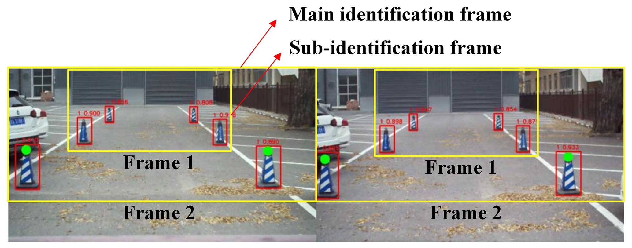
As depicted in Fig. 5, the image identification process consists of two identification frames: the main identification frame (Frame 1) and the sub-identification frame (Frame 2). Frame 1 is used to identify the 3D coordinates of the current marker feature points, while Frame 2 is used as a preparatory frame to identify the marker simultaneously. However, Frame 2 does not extract the 3D coordinates of the marker. Only if the marker in Frame 1 is about to leave the field of view does Frame 2 start to play the role of Frame 1. The identification process repeats until the last marker leaves the field of view.

Figure 5 Image feature point recognition effect diagram.

2.2.2 Kinematic decoupling method

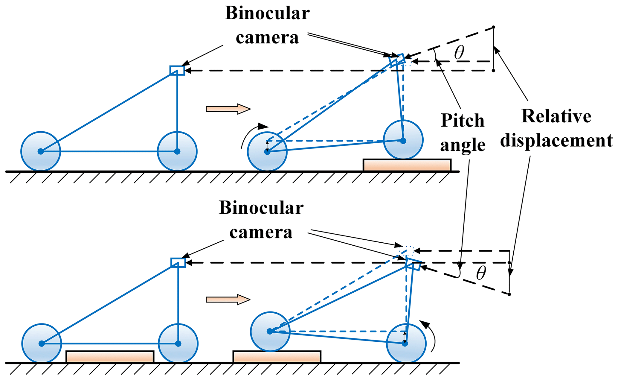
Taking a rectangular cross-section speed bump as an example, the dynamic response of the vehicle and the change in camera field of view, which are caused by low-frequency longwave road unevenness excitation, are analyzed. To figure out the vibration response of the vehicle during operation, two specific cases were designed. The two cases are shown vividly in Fig. 6. In the first case, when the front wheels of the vehicle are fully lifted, the body will undergo a coupled motion consisting of the translation of the front wheels and rotation around the rear wheels. Due to the camera being firmly connected to the vehicle body, this coupled motion is also contained in the movement of the camera. Similarly, in the second case, when the rear wheels of the vehicle are fully lifted, the camera contains a coupled motion consisting of the translation of the rear wheels and rotation around the front wheels during the operation. Therefore, the body vibration and camera motion caused by the low-frequency longwave unevenness excitation are consistently coupled with the bounce and pitch responses.

Figure 6 Kinematic rigid body model for body vibration.

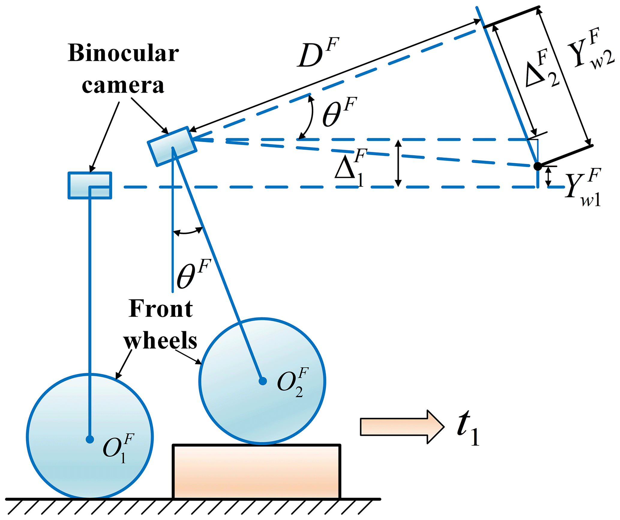
With this in mind, the vehicle can be simplified to a rigid body model, as shown in Fig. 7, when the front wheels are lifted, where $O_{\mathrm{1}}^{\mathrm{F}}$ is the center of the front wheels at the initial state of the vehicle and $O_{\mathrm{2}}^{\mathrm{F}}$ is the center of the front wheels as they are fully moving above the speed bump. Before the front wheels touch the speed bump, according to the binocular measurement principle, the vertical distance (normal projection distance) between the reference mark and the camera optical axis is $Y_{\mathrm{w}\mathrm{1}}^{\mathrm{F}}$. In addition, when the front wheels are above the speed bump, the reference mark moves below the camera optical axis. At this moment, the vertical distance between the reference mark and the camera optical axis is $Y_{\mathrm{w}\mathrm{2}}^{\mathrm{F}}$. θ^F is the camera rotation angle, ${\mathrm{\Delta }}_{\mathrm{1}}^{\mathrm{F}}$ is the camera's vertical displacement, ${\mathrm{\Delta }}_{\mathrm{2}}^{\mathrm{F}}$ is the camera's pitch displacement and D^F is the corresponding depth of the reference mark at moment t₁. Defining the camera rotation counterclockwise as positive and clockwise as negative, the body vibration is decoupled as follows:

$$\begin{array}{}\text{(3)}& \left\{\begin{array}{lcl}{\mathrm{\Delta }}_{\mathrm{2}}^{\mathrm{F}}& =& D^{\mathrm{F}}\tan {\mathit{\theta }}^{\mathrm{F}},\\ {\mathrm{\Delta }}_{\mathrm{1}}^{\mathrm{F}}& =& \left(Y_{\mathrm{w}\mathrm{2}}^{\mathrm{F}}-{\mathrm{\Delta }}_{\mathrm{2}}^{\mathrm{F}}\right)\cos {\mathit{\theta }}^{\mathrm{F}}+Y_{\mathrm{w}\mathrm{1}}^{\mathrm{F}}.\end{array}\right.\end{array}$$

In Eq. (3), θ^F is measured by the IMU and $Y_{\mathrm{w}\mathrm{1}}^{\mathrm{F}}$, $Y_{\mathrm{w}\mathrm{2}}^{\mathrm{F}}$ and D^F are calculated by the binocular measurement principle. Solving this system of equations, the vertical displacement ${\mathrm{\Delta }}_{\mathrm{1}}^{\mathrm{F}}$ of the camera can be obtained for each moment.

Figure 7 Simplified model of the front wheels over the speed bump.

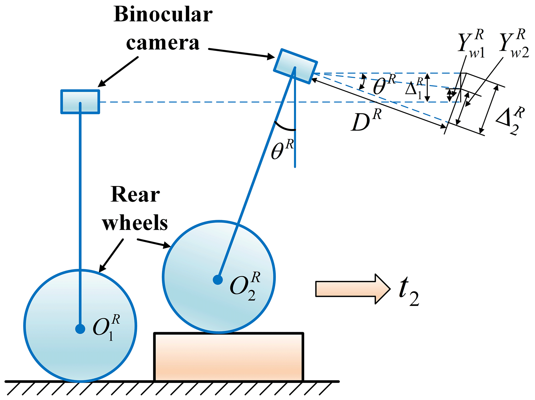
Similarly, when the rear wheels of the vehicle are lifted, the vehicle is simplified to a rigid body model as shown in Fig. 8, where $O_{\mathrm{1}}^{\mathrm{R}}$ is the center of the rear wheels at the initial state of the vehicle and$O_{\mathrm{2}}^{\mathrm{R}}$ is the center of the rear wheels as the rear wheels are fully moving above the speed bump. The body vibration is decoupled as follows:

$$\begin{array}{}\text{(4)}& \left\{\begin{array}{lcl}{\mathrm{\Delta }}_{\mathrm{2}}^{\mathrm{R}}& =& D^{\mathrm{R}}\tan {\mathit{\theta }}^{\mathrm{R}},\\ {\mathrm{\Delta }}_{\mathrm{1}}^{\mathrm{R}}& =& \left({\mathrm{\Delta }}_{\mathrm{2}}^{\mathrm{R}}-Y_{\mathrm{w}\mathrm{2}}^{\mathrm{R}}\right)\cos {\mathit{\theta }}^{\mathrm{R}}+Y_{\mathrm{w}\mathrm{1}}^{\mathrm{R}}.\end{array}\right.\end{array}$$

In Eq. (4), $Y_{\mathrm{w}\mathrm{1}}^{\mathrm{R}}$ is the vertical distance between the reference mark and the camera optical axis before the rear wheels of the vehicle touch the speed bump and $Y_{\mathrm{w}\mathrm{2}}^{\mathrm{R}}$ is the vertical distance between the reference mark and the camera optical axis when the rear wheels of the vehicle are completely above the speed bump. θ^R is the camera rotation angle. ${\mathrm{\Delta }}_{\mathrm{1}}^{\mathrm{R}}$ is the vertical displacement of the camera. ${\mathrm{\Delta }}_{\mathrm{2}}^{\mathrm{R}}$ is the camera's pitch displacement. D^R is the corresponding depth of the reference mark at moment t₂. Consequently, the system of equations can be solved to obtain the vertical displacement ${\mathrm{\Delta }}_{\mathrm{1}}^{\mathrm{R}}$ of the camera for each moment.

Figure 8 Simplified model of the rear wheels over the speed bump.

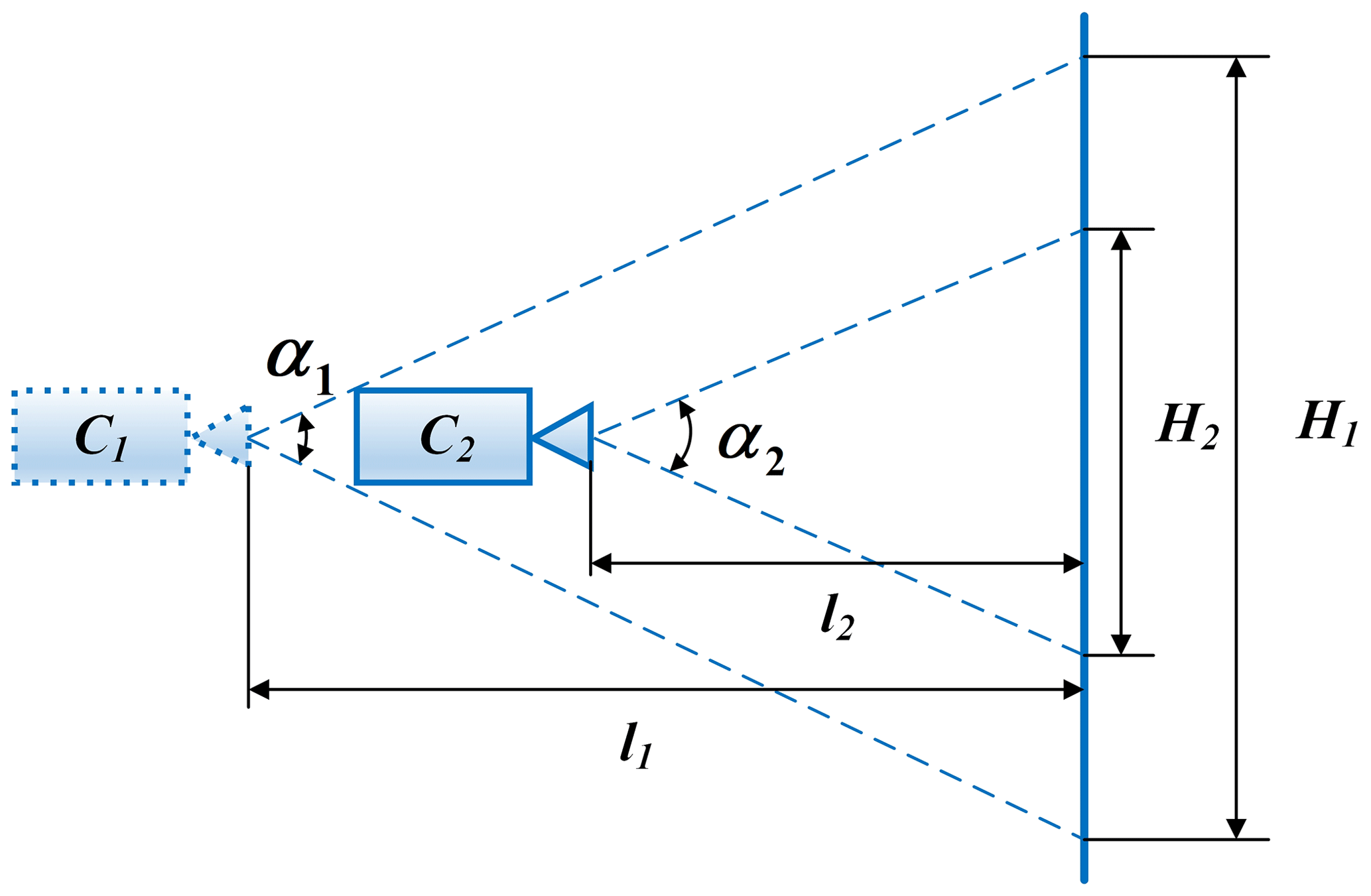
During the process of the camera moving with the vehicle, the field of view of the camera changes with the distance, as shown clearly in Fig. 9. The position of the camera moves with the vehicle from C₁ to C₂ and the distance from the camera to the reference changes from l₁ to l₂. Correspondingly, the height (H₁ and H₂) occupied by the reference within the camera's field of view also changes. Therefore, the camera's field of view angle (α₁ and α₂) can be expressed as

$$\begin{array}{}\text{(5)}& \left\{\begin{array}{ccc}\frac{H_{\mathrm{1}}}{l_{\mathrm{1}}}& =& {\mathit{\alpha }}_{\mathrm{1}},\\ \frac{H_{\mathrm{2}}}{l_{\mathrm{2}}}& =& {\mathit{\alpha }}_{\mathrm{2}}.\end{array}\right.\end{array}$$

During the vehicle operation, since the camera lens parameters do not change, the field-of-view angles of the camera maintain an equal relationship – that is, α₁=α₂ – then the following applies:

$$\begin{array}{}\text{(6)}& {\displaystyle \frac{H_{\mathrm{1}}}{l_{\mathrm{1}}}}={\displaystyle \frac{H_{\mathrm{2}}}{l_{\mathrm{2}}}}=k,\end{array}$$

where k is the proportionality coefficient between the camera field of view and distance, which is expressed as the ratio of the objects in front of the camera to the whole field of view of the camera. The camera's vertical displacement, ${\mathrm{\Delta }}_{\mathrm{1}}^{\mathrm{F}}$ and ${\mathrm{\Delta }}_{\mathrm{1}}^{\mathrm{R}}$, also contain the proportional relationship, so the real vertical vibration displacement (Δ_F and Δ_R) of the body should be

$$\begin{array}{}\text{(7)}& \left\{\begin{array}{lcl}{\mathrm{\Delta }}_{\mathrm{F}}& =& {\mathrm{\Delta }}_{\mathrm{1}}^{\mathrm{F}}\times k,\\ {\mathrm{\Delta }}_{\mathrm{R}}& =& {\mathrm{\Delta }}_{\mathrm{1}}^{\mathrm{R}}\times k.\end{array}\right.\end{array}$$

Figure 9 Schematic diagram of the field of view and distance.

3 Modal simulation analysis

In order to find out what the relationship between the modal parameters of the suspension system and the faults is, a 7-degree-of-freedom (DOF) dynamics model of the whole vehicle was established. Subsequently, the time domain response signal of road unevenness was simulated using MATLAB software. This simulated signal was then input into both normal and faulty dynamics models to obtain the vibration response signals of the body. Finally, these vibration signals were analyzed by SSI to obtain the correlation between the modal parameters and suspension faults. The flowchart of the simulation analysis is presented in Fig. 10.

Figure 10 Schematic diagram of simulation analysis.

3.1 7-DOF vehicle model and its modal parameters

The whole vehicle is simplified to a 7-DOF model, including 3 DOFs for the body – bounce (z), pitch (θ) and roll (φ) – and 4 DOFs for the wheels (z₁, z₂, z₃, z₄). The details of the model are shown in Fig. 11. The model is mainly composed of body mass, under-spring mass, suspension springs and dampers. The body mass is simplified to m₀; the unsprung mass is simplified to m₁, m₂, m₃ and m₄; the suspension spring stiffness and damper damping coefficients are represented by k₁, k₂, k₃ and k₄ and c₁, c₂, c₃ and c₄, respectively; and the tire stiffness is represented by k_t1, k_t2, k_t3 and k_t4. The damping value of the wheels is not considered to have a negligible effect on the results (Hrovat, 1988). The vehicle's parameters are shown in Table 1.

Figure 11 7-DOF model of the whole vehicle.

Table 1 Vehicle component parameters.

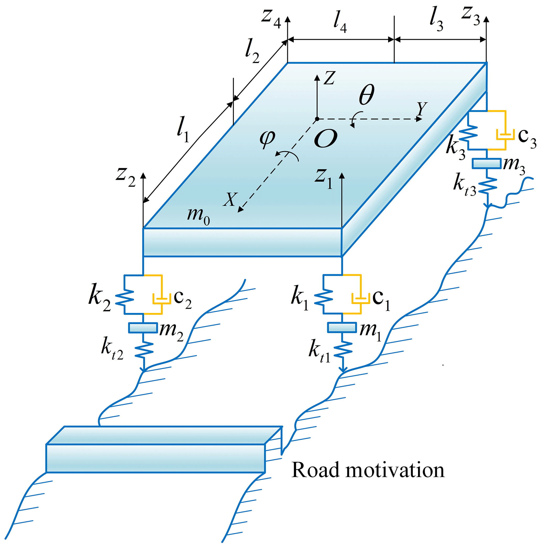
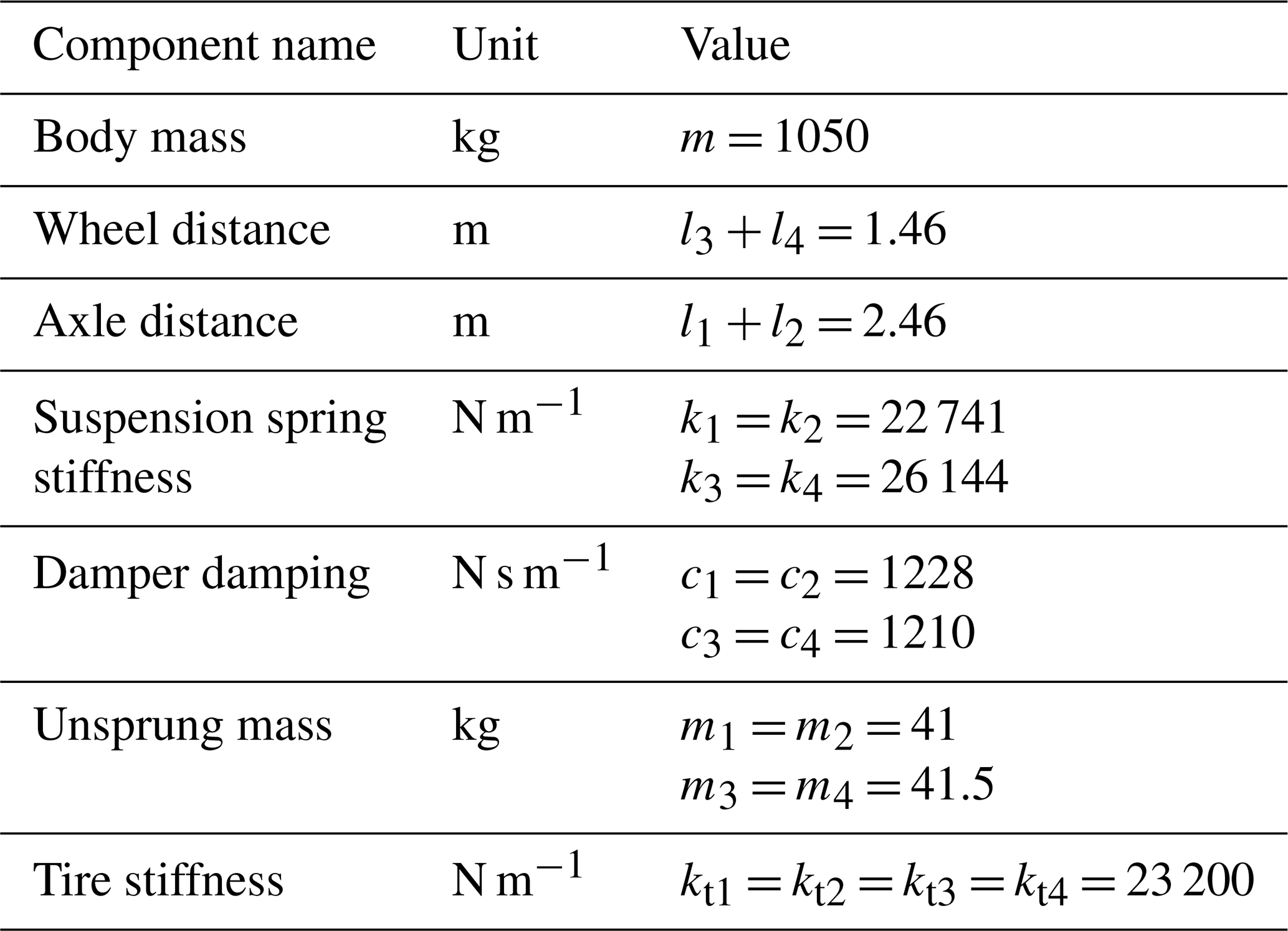
Figure 12 shows the simulation results of road surface unevenness. The data are prepared according to a recent International Organization for Standardization (ISO) report on measurement data of mechanical vibration road surface profiles (GB/T 7031-2005/ISO 8608:2016). In particular, Fig. 12a shows the standard class B road surface unevenness signal, Fig. 12b shows the simulated pulse signal and Fig. 12c shows the superimposed road surface unevenness simulation signal. The solid line in the figure represents the road surface unevenness signal of the left front wheel, and the dashed line indicates surface unevenness signal of the left rear wheel. After inputting the superimposed constructed road surface unevenness signal into the 7-DOF model, the vertical vibration signal of the body can be obtained through simulation.

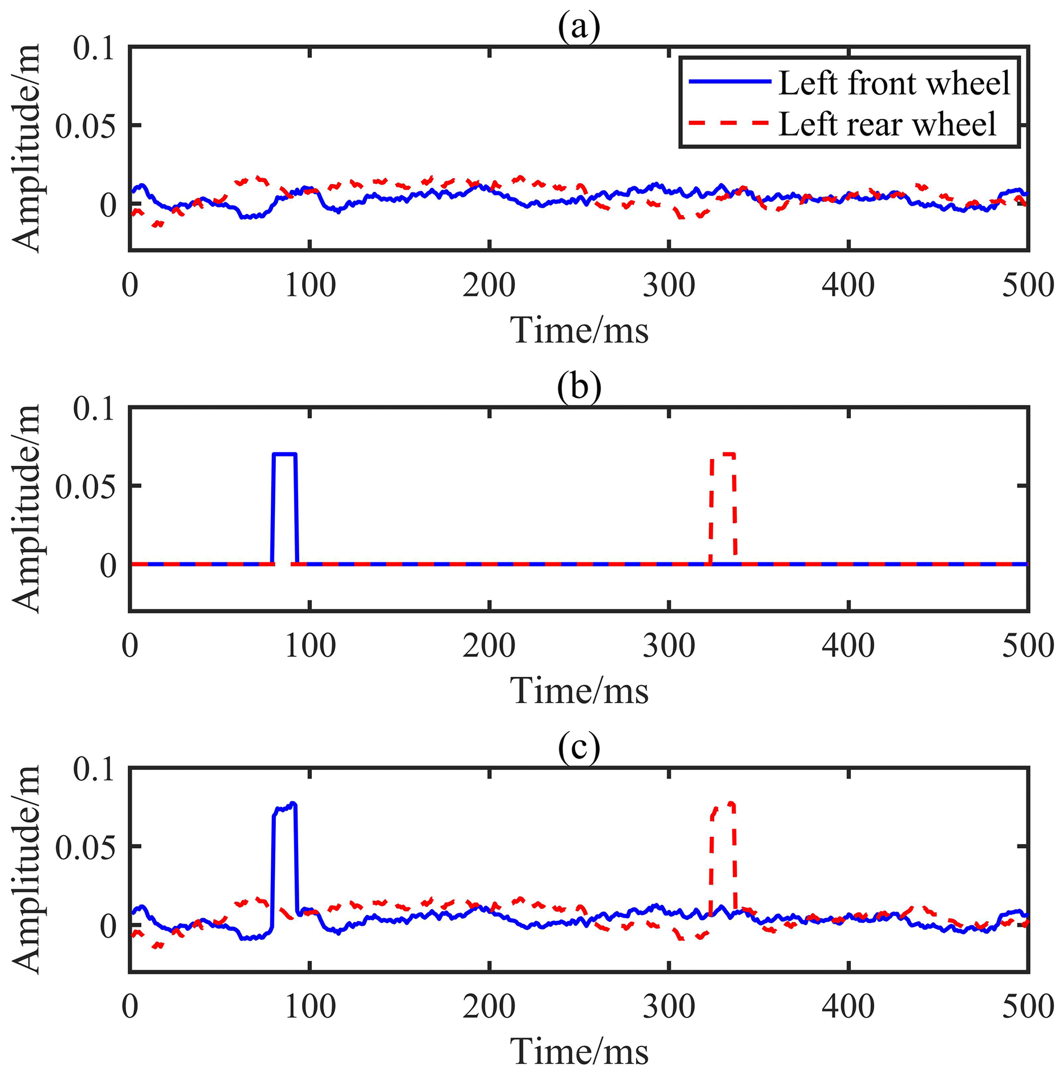
Figure 12 Simulation results of road surface unevenness: (a) standard class B road surface unevenness signal, (b) simulated pulse signal and (c) simulated road surface unevenness signal.

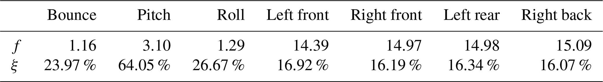
Stochastic subspace identification (SSI) is a method of identifying structural modal parameters based on environmental excitations. The changes in modal parameters identified by SSI can be used for type identification and level determination of the fault caused by suspension failures. The accuracy of the SSI-based diagnostic method relies only on the accurate identification of abnormal changes in modal parameters compared to the baseline. This method offers excellent portability that only requires baseline parameter modifications and recalibrations for different vehicles. At present, there are two primary stochastic subspace methods: data-driven subspace-based methods and covariance-based subspace methods. In this paper, an average correlation signal-based SSI (ACS-SSI) method is applied, which is an improvement on the covariance-based methods (Chen et al., 2015b)​​​​​​​. The ACS-SSI method has the particular advantage of combining high computational robustness and efficiency. The identified modal parameters primarily include natural frequency, mode shape and damping ratio. By establishing the SSI modal feature identification algorithm in MATLAB, the modal parameters of the whole vehicle system were successfully identified. The information on the characteristics of the whole vehicle dynamics model is detailed in Table 2.

Table 2 Information on the characteristics of vehicle dynamics model.

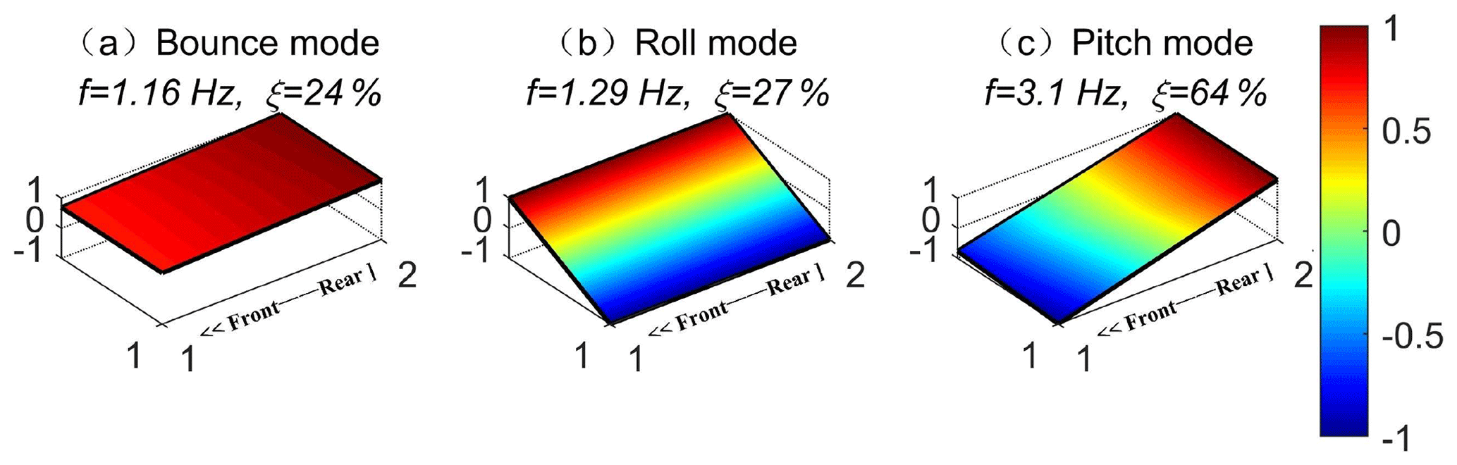
The mode shape diagrams of the body in the bounce, pitch and roll modes are shown in Fig. 13. During regular operation of the vehicle, the mode shapes of its left and right sides are always the same. Moreover, the characterization of the roll mode shape is not obvious. Therefore, fault diagnosis can be achieved by analyzing the changes in mode shapes of two types: bounce and pitch.

Figure 13 Mode shapes of the body.

3.2 Influence of suspension faults on modal parameters

During the long-term operation of a vehicle, various load conditions and environmental factors can lead to suspension faults. Therefore, the modal parameters (natural frequency, damping ratio and mode shape) of the suspension system under the influence of different fault types are simulated in MATLAB. Subsequently, the effects of different suspension faults on the modal parameters can be obtained.

3.2.1 Influence of spring stiffness changes on modal parameters

To investigate the influence of spring stiffness on the modal parameters, the stiffness of the right rear spring was changed from 0 % to 50 % in MATLAB to simulate the spring failure. The simulation results are presented in Fig. 14. The blue line represents the bounce mode, the brown line represents the pitch mode, and the orange line represents the roll mode.

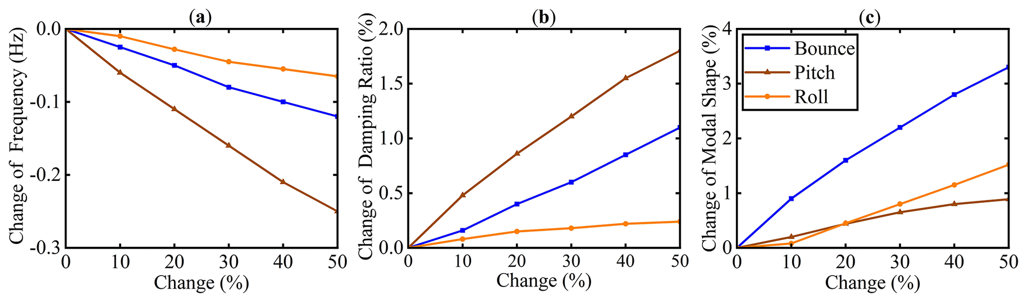
Figure 14 Changes in modal parameters caused by a right rear suspension spring fault: (a) natural frequency, (b) damping ratio and (c) mode shape.

It can be seen from Fig. 14a that as the spring stiffness decreases, the natural frequencies of all three modes decrease to different degrees. The pitch mode decreases by 0.25 Hz and changes the most as the amplitude changes in the bounce mode and roll mode are lower. In Fig. 14b, the damping ratios of the three modes increase significantly, in which the pitch mode changes the most, followed by bounce mode and roll mode. Compared to the first two modal parameters, the mode shapes vary more significantly, with the rate of change in the bounce mode reaching 3 %.

Figure 15 presents the simulation results of Hamed (2016) regarding the effect of spring stiffness variation on modal parameters. The spring stiffness was reduced from 100 % of the original value to 80 % to simulate suspension failure. Despite the differences in vehicle suspension parameters between the two studies, the trend of modal parameters for both simulations is consistent, confirming the reasonability of the modeling in this paper.

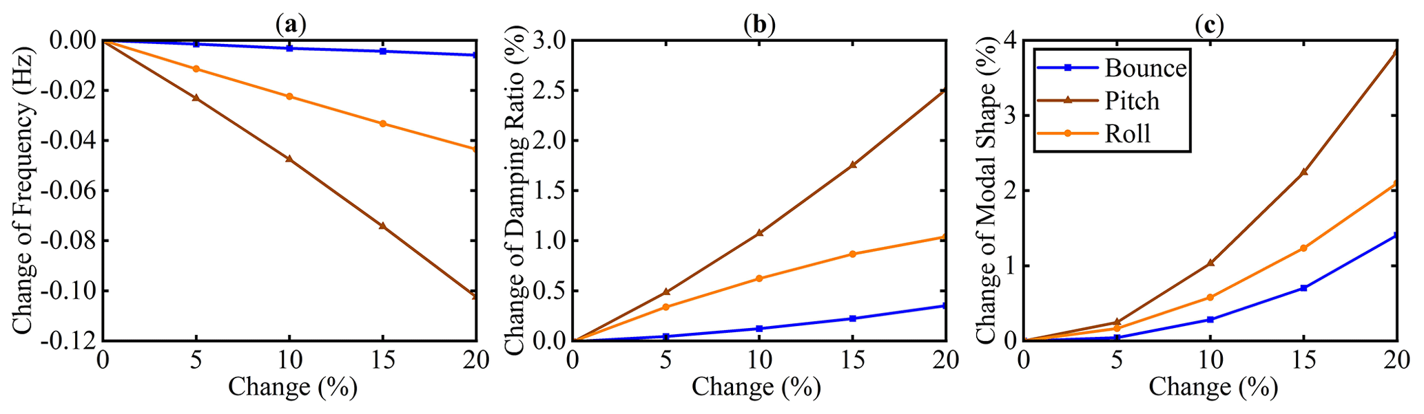
Figure 15 Changes in modal parameters caused by a right rear suspension spring fault: (a) natural frequency, (b) damping ratio and (c) mode shape (adapted from Hamed, 2016).

3.2.2 Influence of damping changes on modal parameters

The damping value of the right rear suspension is changed from 0 % to 50 % in MATLAB to analyze the trend of the modal parameters at each order. Figure 16 demonstrates the changes in modal parameters when the right rear damper damping is faulty. With the damping value of the damper decreasing, the natural frequency and damping ratio of the three modes show a decreasing trend, while the mode shape shows an increasing trend.

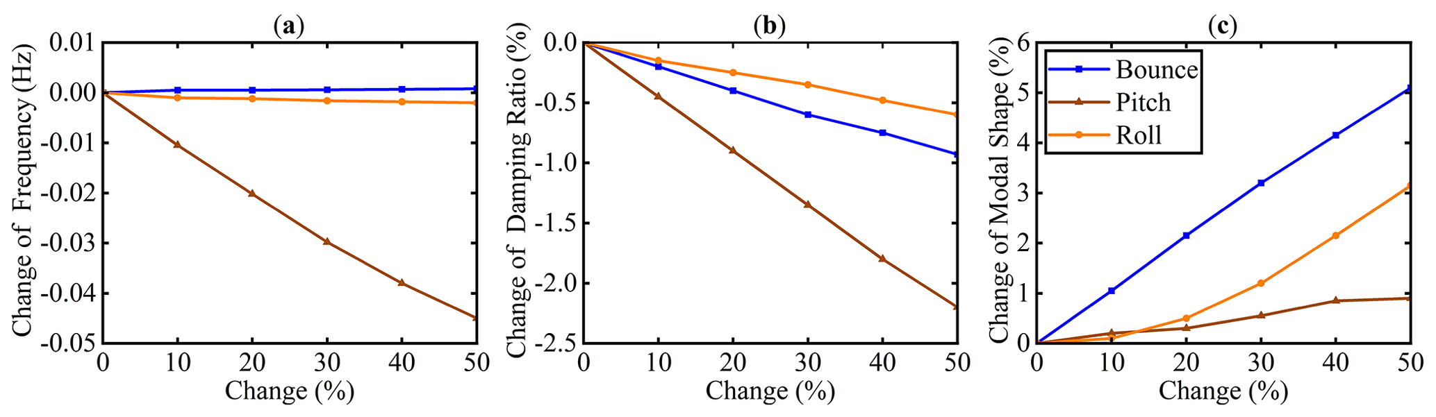
Figure 16 Changes in modal parameters caused by damping failure of a right rear suspension: (a) natural frequency, (b) damping ratio and (c) mode shape.

3.2.3 Influence of tire pressure changes on modal parameters

In MATLAB, the stiffness of the right rear tire is changed from 0 % to 50 % to indirectly simulate tire pressure faults. From Fig. 17, it can be seen that as the tire pressure drops, the natural frequency and damping ratio in all three modes decrease, especially in the pitch mode, where the natural frequency and damping ratio decrease the most. The rate of change in the mode shape increases as the tire pressure decreases.

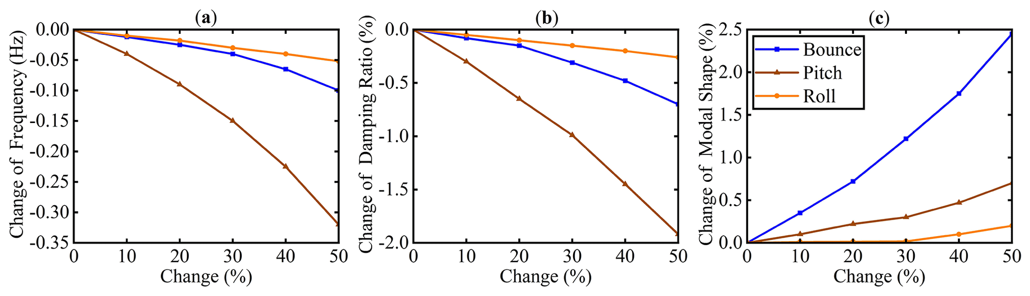
Figure 17 Changes in modal parameters caused by the reduction in tire pressure of a right rear tire: (a) natural frequency, (b) damping ratio and (c) mode shape.

In summary, when some typical components of a suspension system fail, all three modal parameters of the system change to varying degrees. However, since the vehicle suspension system is a damped vibration system with a high damping value, accurately measuring it with existing testing methods can be challenging. As a result, the practical damping ratio of the system is more difficult to accurately reflect on. On the other hand, the mode shape is considered an eigenvector, with a dimensionless value that varies more noticeably. Therefore, among the three modal parameters, much attention needs to be paid to the changes in mode shape, which is used as a detection indicator for suspension system fault diagnosis.

4 Experiment study

4.1 Test design and test program

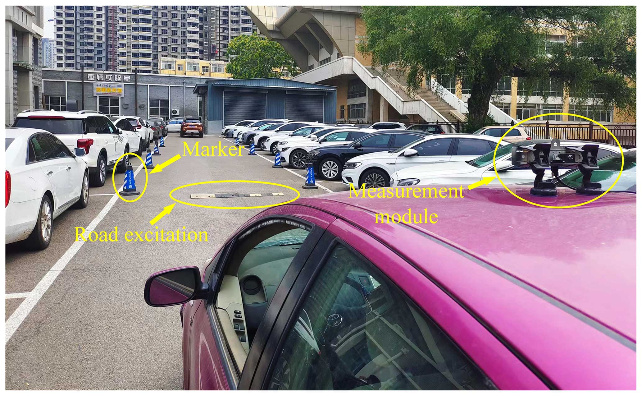
The test system comprises a measurement module, road excitation, markers and vehicle, as shown in Fig. 18. The measurement module consists of a binocular camera and an IMU. To acquire the vehicle vibration response caused by road excitation in the frequency interval of 0.5–30 Hz, the image resolution of the binocular camera was set to 1280 × 480 pixels, and the acquisition frame rate was set to 90 fps. It is equipped with an 8 mm focal-length lens, and the baseline is set to 130 mm in the test. The pitch angle is acquired synchronously using an IMU with a sampling frequency set to 400 Hz. The road excitation used in the test is a rectangular speed bump with a height of 70 mm. Standard road pile barrels are used as markers. The test vehicle is an ordinary passenger car. The binocular camera is fixed horizontally in the middle of the body, and the IMU is fixed at the center of the camera pitch axis. First of all, it is important to select a straight and less disturbed road, set up road excitation and markers at a distance of 10 m from the vehicle. The vehicle then passes through the road excitation at three speeds, i.e., 5, 10 and 20 km h⁻¹, respectively. When the rear wheels of the vehicle leave the road excitation, a rapid braking operation is performed to ensure safety of the test system and experimental personnel.

Figure 18 Diagram of the test system.

In order to verify the effectiveness of the suspension fault identification algorithm, tests were conducted under various suspension faults. The suspension faults were identified by analyzing the body vibration response caused by random road unevenness excitation. Therefore, real test programs were designed for spring failure (reduced stiffness), damper failure (reduced damping) and tire failure (reduced pressure) condition, respectively. The test cases are detailed as follows:

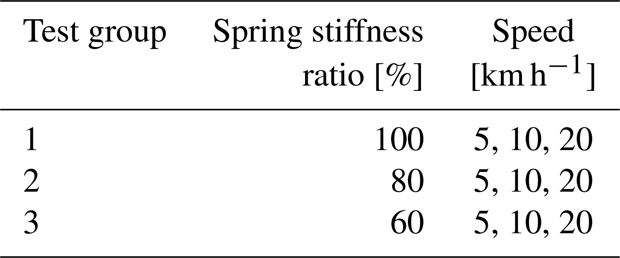
In the first test case, named Case 1, the spring failures were simulated by changing the effective number of turns of the right rear suspension spring. The original spring was replaced by springs with 80 % and 60 % of their stiffness, respectively. In addition, the vehicle passes through the rectangular speed bump at 5, 10 and 20 km h⁻¹, respectively. The grouping situations are presented in Table 3.

Table 3 Spring failure test.

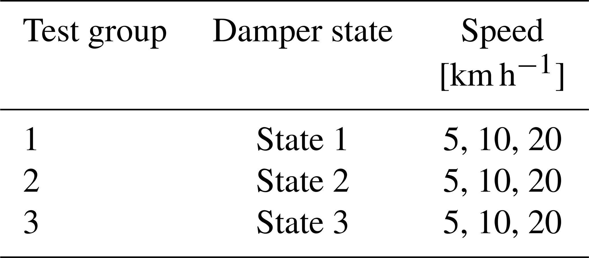
In the second case (Case 2), the right rear suspension damper was replaced with an adjustable damping damper. The adjustable damping damper is set to the three states, with State 3 being the baseline state. The damping values from State 3 to State 1 are 100 %, 80 % and 60 %, respectively. The test groups are shown in Table 4.

Table 4 Damper failure test.

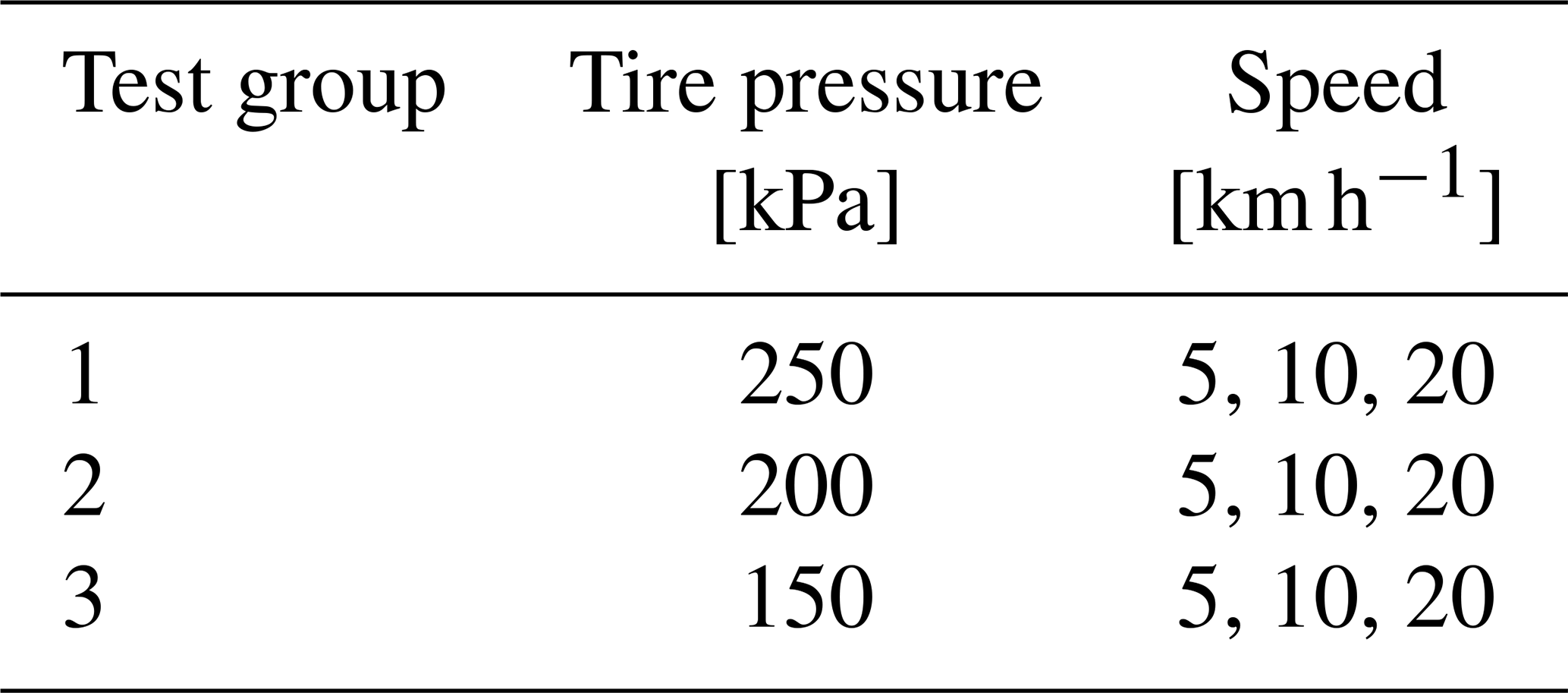
In the third test case (Case 3), tire failures were simulated by deflating the right rear tire. The reduced tire pressure was divided into two levels, as shown in Table 5, which are 80 % and 60 % of the standard tire pressure.

Table 5 Tire pressure failure test.

4.2 Verification of body vibration response

When the vehicle passes through the rectangular speed bump at different speeds, the body will generate various degrees of vertical vibration. As shown in Fig. 19, the solid blue line represents the vertical displacement measured by the binocular camera and the dashed red line represents the vertical displacement measured by the IMU. Moreover, the first and second wave peaks in the figure correspond to the displacements caused by the front and rear wheels being completely above the rectangular speed bump, respectively.

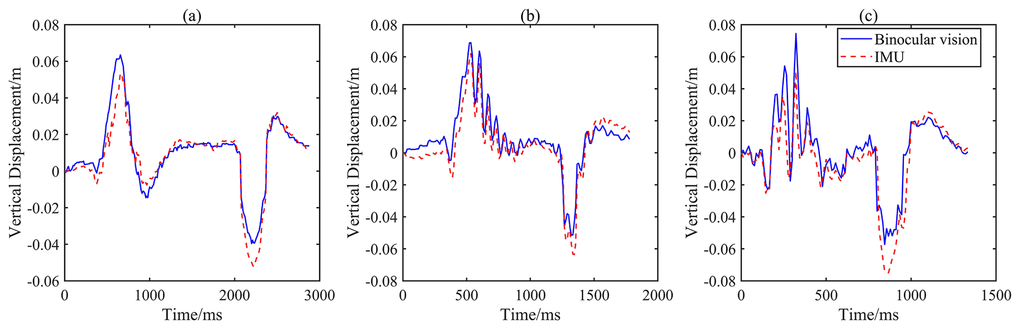
Figure 19 Vertical displacement-time curves at different speeds: (a) 5 km h⁻¹ vehicle speed, (b) 10 km h⁻¹ vehicle speed and (c) 20 km h⁻¹ vehicle speed.

It can be seen from Fig. 19 that the impulse responses of the binocular vision and IMU measurement curves are well synchronized. Comparing the curves at different speeds, the impulse response time becomes shorter and the peak amplitude increases as the vehicle speed increases, which is consistent with the reality that higher travel speeds cause increased vibration.

When the front wheels are above the speed bump, the vertical displacement of the reference mark measured by the binocular camera contains two components: the deflection displacement (Δ₂) and the vertical jump displacement (Δ₁). In order to facilitate the comparison of the amplitudes of the two displacements, the vertical displacement Y_w measured by the binocular camera is inverted. Since the direction of camera deflection is consistent with the direction of the vertical jump, the amplitude of the binocular measurement data, max(Y_w), is larger than that of the IMU measurement data, max(Δ₂). However, when the rear wheels are above the speed bump, the deflection of the camera is in the opposite direction to the vertical jump, resulting in the absolute value of the valley, min(Y_w), of the binocular measurement data being smaller than that of the valley, min(Δ₂), of the IMU measurement data. Based on the principle of kinematic decoupling of the body, the vertical displacement of the vehicle across the speed bump is calculated as the cosine of the difference between the displacements measured by the two devices. Furthermore, the calculated results are all positive.

As shown in Fig. 20, the solid line is the body vertical vibration curve measured based on binocular vision and kinematic decoupling, while the dashed line represents the vertical vibration obtained by simulation. It can be clearly seen that the impulse responses of the two curves are well synchronized. Since the camera is installed in the middle of the front and rear axles of the vehicle, the peak vertical vibration of the body should be half of the height of the rectangular speed bump, according to the similar triangle theory. As a result, when the front and rear wheels of the vehicle drive over the speed bump, both the measured data and the simulated data show a vertical vibration amplitude of about 35 mm, which confirms the validity of the proposed algorithm.

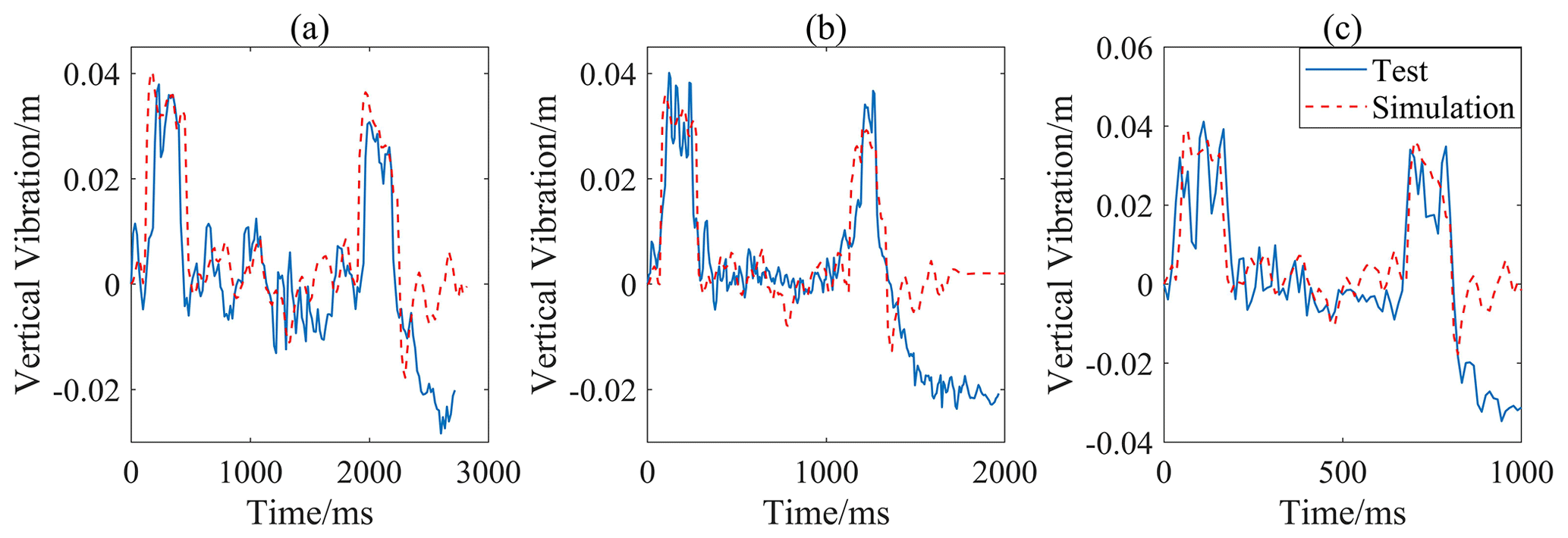
Figure 20 Simulated and measured body vertical vibration-time curves: (a) 5 km h⁻¹ vehicle speed, (b) 10 km h⁻¹ vehicle speed and (c) 20 km h⁻¹ vehicle speed.

However, it should be noted that after the second wave peak in Fig. 20, the measured vibration displacement curve shows a sharp decline. Limited to the length of the test road, emergency braking was applied to the vehicle when the rear wheels left the speed bump. Hence, the data after the second peak show a large deviation. This can be optimized in the future by improving the test program.

4.3 Test and result analysis

Due to the requirement for random excitation data in the SSI modal identification method, the vibration signals of a vehicle traveling on a normal road without road excitation were used as the data source for the analysis of the results. Additionally, since there were only minor differences between the test data at various speed conditions, the 20 km h⁻¹ speed condition was chosen for the analysis of the results.

4.3.1 Spring failure

First, the mode shapes of non-failed and failed springs were analyzed. Moreover, comparing the mode shapes for each condition in Case 1. The results are shown in Fig. 21. Figure 21a and b show the mode shapes of bounce and pitch modes for the baseline condition, Fig. 21c and d show the mode shapes of bounce and pitch modes for 80 % spring stiffness, and Fig. 21e and f show the mode shapes of bounce and pitch modes for 60 % spring stiffness. It can be seen from the figures that as the spring stiffness decreases, the natural frequencies in both bounce and pitch modes show a decreasing trend, but the natural frequency changes more obviously in the pitch mode. Besides, the change rate of the mode shape in the bounce mode is larger than that of pitch mode. These changes verify the results obtained from the simulation.

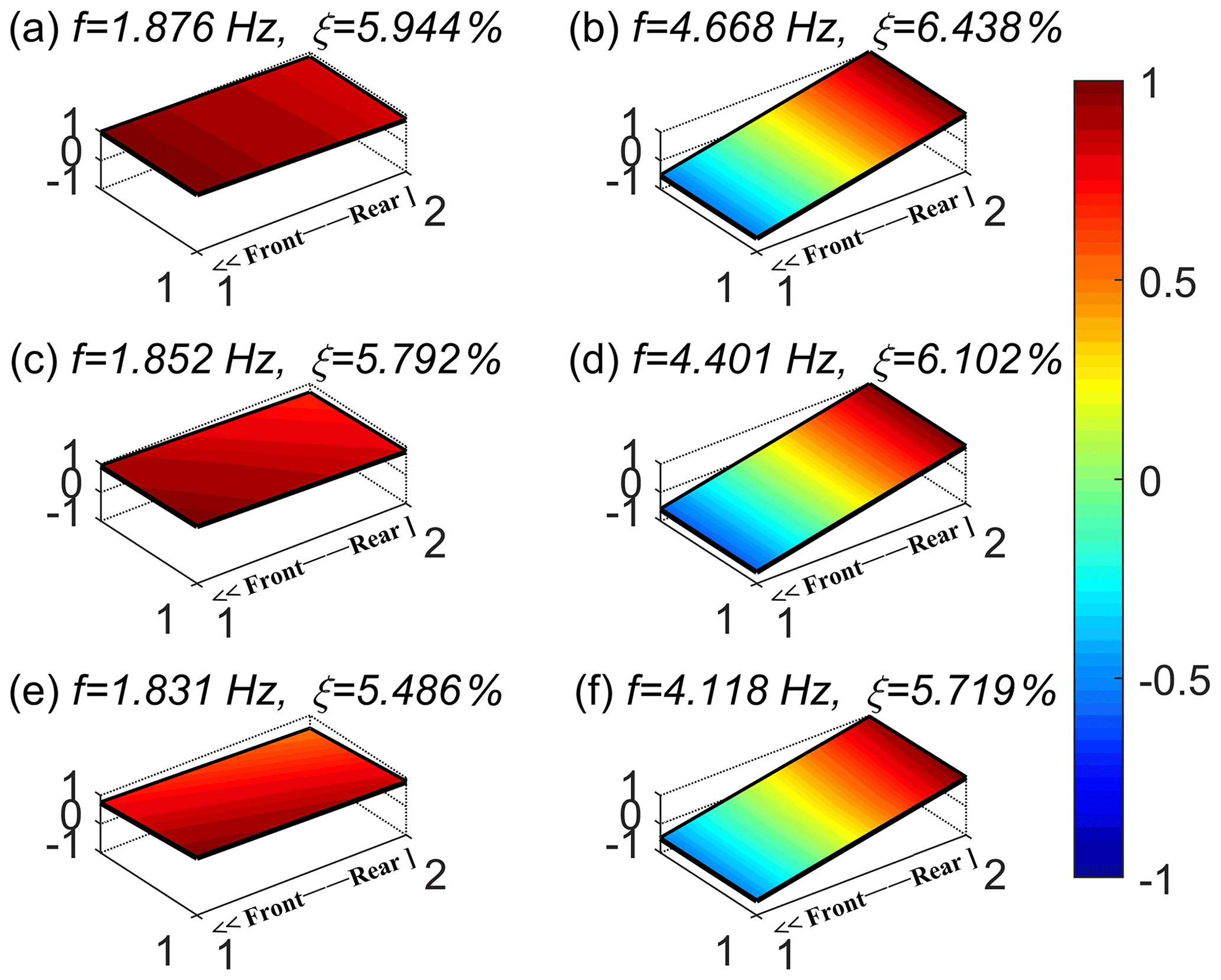
Figure 21 Mode shapes for different spring stiffness: (a, c, e) bounce mode and (b, d, f) pitch mode.

Figure 22 shows the diagnostic results for the suspension spring failure based on the vibration sensor data (Li et al., 2017). Figure 22a and b show the mode shapes of bounce and pitch modes for the baseline condition. Figure 22c and d show the mode shapes of bounce and pitch modes for 80 % spring stiffness. It can be seen from Fig. 22 that as the spring stiffness decreases, the natural frequencies of the bounce and pitch modes show the same decreasing trend as in this paper. This confirms the validity of the diagnostic results of the proposed method regarding suspension stiffness failure.

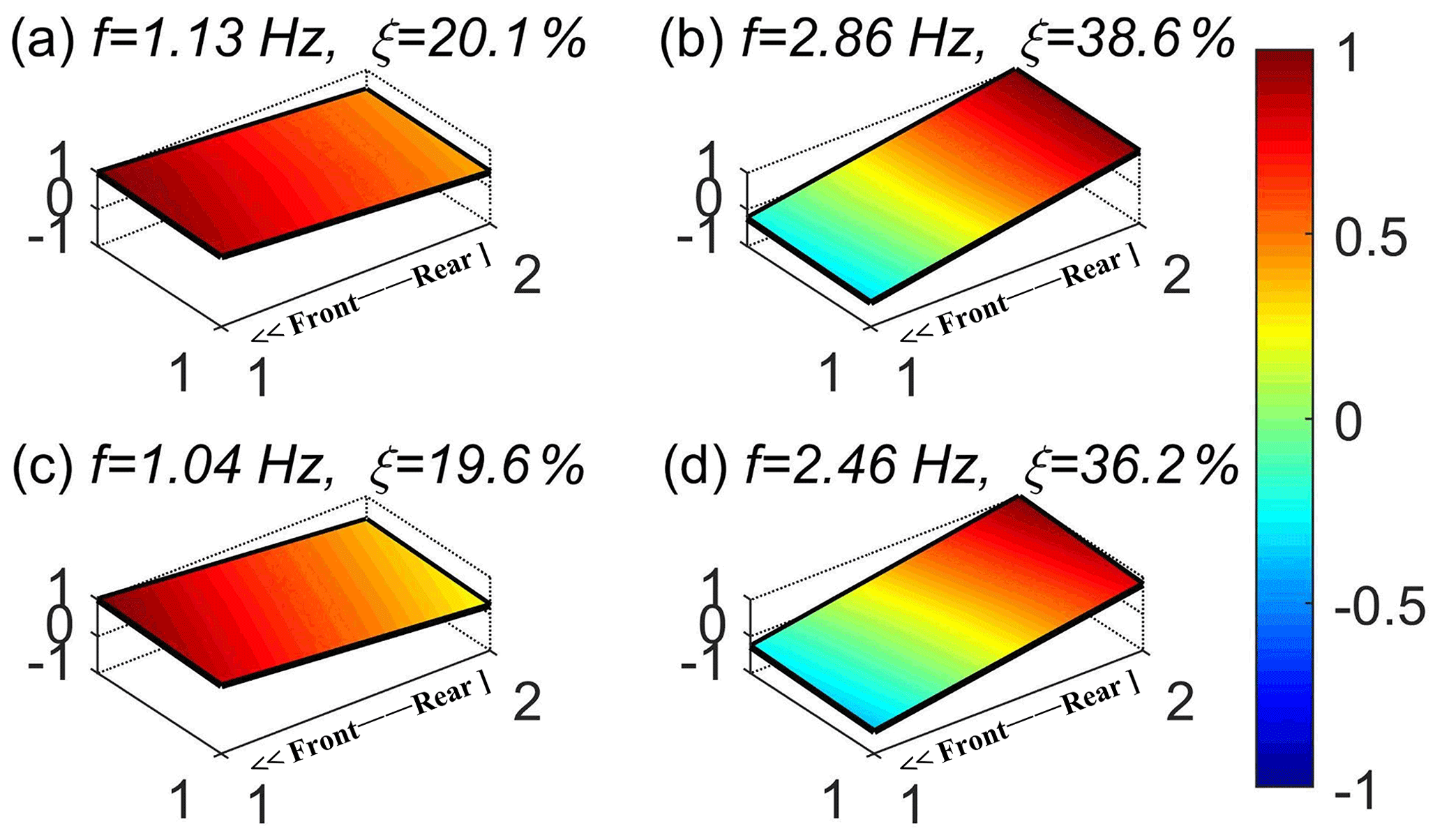
Figure 22 Modal parameters for baseline and fault states: (a, c) bounce mode and (b, d) pitch mode (adapted from Li et al., 2017).

4.3.2 Damper failure

Figure 23 shows the mode shapes of the damper damping failures. It can be seen from the figure that as the damping value of the damper decreases, the natural frequencies in both bounce and pitch modes decrease, with the pitch mode showing a larger decrease. The mode shape changes little in the bounce mode, while the mode shape changes more obvious in the pitch mode. In addition, the damping ratio in the bounce and pitch modes changes more significantly, which means that this signal can be used as an indicator for the identification of the damper damping faults.

Figure 23 Mode shape for different damping: (a, c, e) bounce mode and (b, d, f) pitch mode.

4.3.3 Tire failure

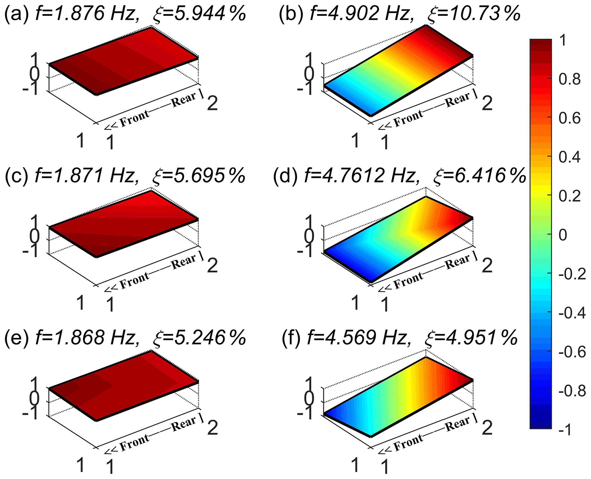
The test results of the vehicle tire pressure failures are shown in Fig. 24. Similar to the results of the spring failure test groups, as the right rear tire pressure decreases, the natural frequencies in both the bounce and the pitch modes show a decreasing trend, and the mode shape in the bounce mode undergoes the most significant changes.

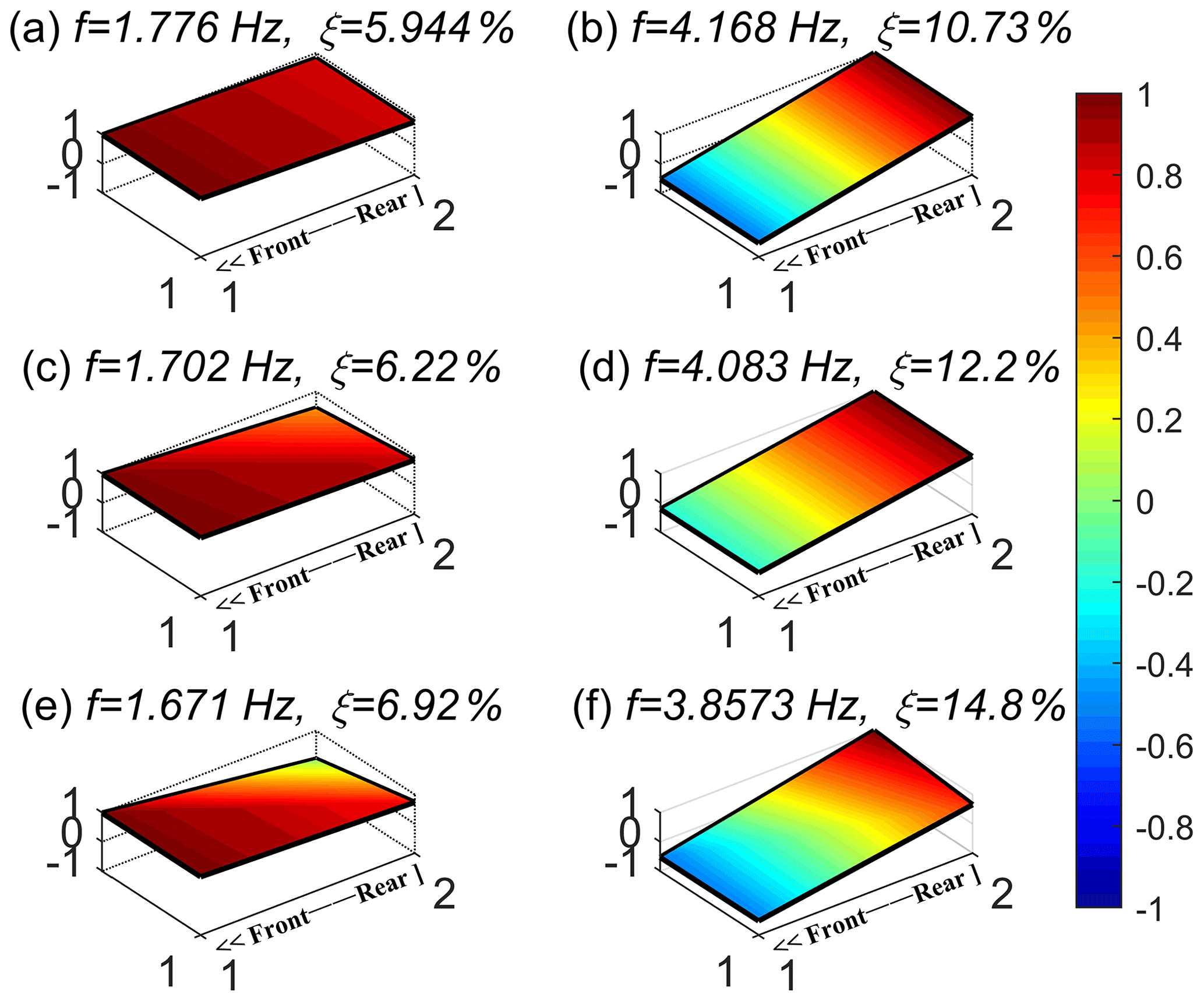
Figure 24 Mode shape diagrams at different tire pressures: (a, c, e) bounce mode and (b, d, f) pitch mode.

4.3.4 Result discussion

The above analysis indicates that the suspension failures would lead to obvious changes in a vehicle's modal parameters (mainly the natural frequencies and mode shapes). Different types of failures will lead to different changes in the modal parameters. By establishing a mapping between faults and modal parameter variations, the identification of the type and degree of suspension faults can be realized. Decreases in spring stiffness, damper damping and tire pressure all lead to a decrease in the natural frequency of the bounce and pitch modes. Compared to the other two types of suspension failure, the damping ratio is more sensitive to damper damping failures. The magnitude of change in modal parameters can characterize the severity of the failures.

The results of real-vehicle experiments and simulation analyses show that the vertical vibration signals of the vehicle can be effectively acquired using binocular vision technology and a kinematic decoupling algorithm. Moreover, the measured vibration signals are highly accurate to reflect the real vibration condition of the vehicle. In combination with the SSI method, it is effective to identify different types and degrees of suspension faults.

5 Conclusions

The main aim of this paper is to develop a real-time monitoring scheme for vehicle suspension systems. For this purpose, a method based on binocular vision and kinematic decoupling was carried out to measure the vehicle's vibration signals. Moreover, these vibration signals were analyzed in combination with the SSI method to monitor suspension faults. By analyzing the changes in suspension modal parameters, the types and degrees of faults in the suspension system were identified and evaluated. Both the simulation analysis and the experimental results provide compelling evidence that this method is effective in vehicle suspension fault diagnosis. The main conclusions can be drawn as follows: visual vibration measurement technology is a novel method that has the ability to effectively extract a vehicle's vertical vibration signals. Moreover, this method has the advantages of real-time measurement and low costs, which overcomes the limitations of traditional measurement methods in terms of error accumulation. In addition, by integrating this functionality using existing cameras, intelligent vehicles can realize the online condition monitoring of suspension and cost-saving in a further step. The proposed method provides an innovative idea for improving the active safety performance of vehicles.

It should be noted that the suspension fault diagnosis method proposed in this paper has some limitations. Firstly, the accuracy of fault diagnosis may be affected by the image quality and camera resolution. Using a high-resolution camera can improve the accuracy of fault diagnosis. Secondly, complex environmental conditions (e.g., light variations, shadows and occlusion) may lead to unstable diagnostic results. It is possible to make the method more adaptable by introducing additional sensors. Thirdly, for more complex suspension faults, it is necessary to combine other fault diagnosis techniques to improve the accuracy and efficiency of fault diagnosis.