Gravity compensation and output data decoupling of a novel six-dimensional force sensor

A shunt three-legged parallel six-dimensional force sensor has been designed for more precise measurement of six-dimensional force/moment information. The theoretical static force model of the sensor was established based on the equivalent of a six-bar closed-loop parallel mechanism. The sensor has been experimentally calibrated under a given external load, and the neural network method has been utilized to nonlinearly fit the experimental data and achieve decoupling. Furthermore, a novel gravity compensation method for the six-dimensional force sensor of the wrist of a robot has been proposed based on the CAD variable geometry method. The positive solution of the position of the parallel robot is simulated through a wire-frame diagram, enabling accurate estimation and correction of the sensor. Experimental validation has confirmed the feasibility of the compensation algorithm.

1 Introduction

Six-dimensional force sensors, which can simultaneously detect all force information in three-dimensional space, are widely utilized in machinery manufacturing, automation, and aerospace due to their comprehensive force measurement information and high measurement accuracy (Zhao et al., 2015; Yin et al., 2005). To fulfill the requirements of precise control in flexible machining assembly and scalpel operations that necessitate force feedback signals, it is essential to endow the sensors with characteristics such as high sensitivity, reliability, and low hysteresis.

Hou et al. (2008) utilized the spiral theory to establish the sensor and constructed a hydrostatic model for it. Chao and Chen (1997) employed the condition number to assess the sensor's performance and developed a novel decoupled wrist force sensor. Jung et al. (2020) designed a novel single-motor-driven flexible-hinge focusing mechanism, which can significantly improve the bending stiffness of the mechanism itself while maintaining excellent flexible axial stiffness for performance optimization. Wu et al. (2013c) conducted a study on the impact of structural parameters on the dynamic characteristics of planar PRRRP (where P represents a prismatic joint and R represents a revolute joint) parallel robots, providing a solution for the selection of structural parameters in parallel mechanisms. Wu et al. (2013a, b) employed a redundant design concept to enhance the kinematic and dynamic performance of the three-degree-of-freedom parallel mechanism, thereby improving its stiffness and load-bearing capacity.

In ideal conditions, a six-dimensional force sensor should only output force in the direction of the input single-dimensional force. However, due to factors such as sensor structure design, processing accuracy, and other issues, inevitably those forces will also be output in other directions, resulting in the greatest extent possible to enhance sensor performance and meet the needs of different fields (Sun et al., 2023). Currently, linear static decoupling and nonlinear static decoupling are the primary decoupling algorithms used for six-dimensional force sensors (Zhu, 2019). By utilizing these decoupling algorithms and formulas, the negative effects of coupling are minimized, thereby improving the measurement accuracy of the sensor and facilitating intuitive output of the components of the externally loaded six-dimensional force through corresponding software that processes experimental data.

During the robot's movement, the zero position of the six-dimensional force sensor undergoes constant shifts due to the consistent variations in its pose and the impact of the gravity acting on the operating tool mounted on the sensor (Pan et al., 2023), ultimately impeding precise robotic control. To ensure accurate measurement of the contact force exerted by the robot's end-effector, it is imperative to conduct zero-point calibration and gravity compensation for the six-dimensional force sensor mounted on the robot's wrist. When robots perform precision tasks such as flexible assembly and flexible machining, it is crucial to accurately sense the six-dimensional force and torque at the contact point between the end-effector and the external environment. This force feedback information is key for the robot to adjust its position and posture in real time and achieve precise operations. However, the gravity of the operating tools can cause deviations in the sensor output values, affecting the perception accuracy. Therefore, gravity compensation for sensors is crucial as it corrects the gravity component, enabling the robot to obtain more accurate information about external forces and improve operational precision.

Nowadays, an increasing number of factories have adopted robots equipped with six-dimensional force sensors on their production lines to enhance efficiency. However, when these sensors become inaccurate, the challenges arise due to their heavy weight, complex structure, and difficulty in disassembly. Field calibration is also problematic, and currently, offline calibration is the primary solution, which is both time-consuming and laborious, significantly affecting the production efficiency of our partner companies.

In response to the urgent needs of our collaborators, our research team has been working on improving the sensor structure to facilitate on-site calibration. We have designed a novel lightweight six-dimensional force sensor with a simple structure, easy disassembly, and convenient replacement for calibration. All components exhibit excellent interchangeability; even if the force-measuring unit becomes damaged, a certain level of measurement accuracy can be maintained without the need for secondary calibration, thus satisfying the demand for uninterrupted production from our partner companies.

2 Sensor structural design

Amidst the perpetual innovation and progression of six-dimensional force sensor technology, the sensor structure has increasingly demonstrated distinctive and varying characteristics.

Cylindrical beam and cross-beam-based six-dimensional force sensors boast high stiffness and a compact structure, yet they are not without their challenges (Payo et al., 2018; Wang et al., 2023). Throughout extended usage, strain gauges are susceptible to environmental factors, potentially compromising the sensor's measurement accuracy. Furthermore, in the event of strain gauge damage, entire sensor replacement is often necessary, significantly elevating operational costs.

The parallel six-dimensional force transducer, represented by the Stewart platform, boasts a high stiffness, making it well suited for measuring heavy loads (Yao et al., 2014). However, the Stewart-type transducer typically comprises six branches of the force-measuring unit and one preloaded branch, resulting in a super-static structure. Consequently, its mechanical analysis and calibration processes are significantly more intricate.

Capacitive six-dimensional force sensors based on microelectromechanical system (MEMS) technology are particularly suitable for precision measurement of small forces/torques (Cai and Yao, 2020), but such sensors are currently more loaded in the production and processing processes, with higher manufacturing costs, making them unsuitable for mass production.

To address the limitations of traditional sensors and meet the requirements of strong load-bearing capacity, lightweight design, high sensitivity, easy disassembly, and convenient replacement, a shunt three-legged parallel six-dimensional force sensor with rigid–flexible hybrid support is proposed.

The structure of the three-legged shunt six-dimensional force sensor proposed in this paper is shown in Fig. 1. Based on the hydrostatic principle of the six-bar closed-loop parallel mechanism, the decomposition of the six-dimensional external loads into forces F₁ and F₂ along the branches. That is, F₁ is balanced by the counterforce provided by the rigid–flexible hybrid bracket and the force-measuring unit. In the sensor branch, the load F₁ is jointly supported by the rigid–flexible hybrid bracket and the force-measuring unit. Notably, the hybrid bracket, with its remarkable stiffness, carries the majority of the load, designated as F₃, which comprises the lion's share of F₁. Meanwhile, the force cell assumes responsibility for a minor portion of the load, designated as F₄. Similarly, F₂ is shared and borne by F₅ and F₆. This innovative load-splitting design brilliantly enhances the sensor's overall measurement range, enabling the utilization of small-range force cells for the accurate measurement of even heavy loads.

Figure 1 New hybrid rigid–flexible sensor bracket.

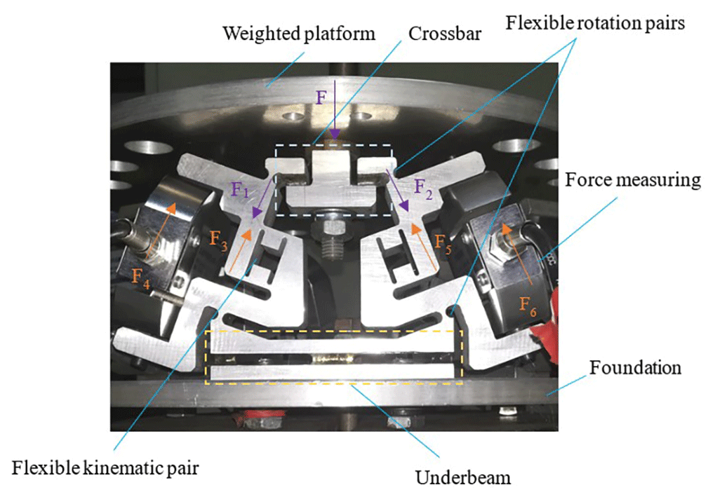
The hybrid rigid–flexible bracket consists of an upper beam, a lower beam, and a symmetrical flexible kinematic pair, which are connected by four flexible rotating pairs. The upper beam is connected to the loading platform through a vertical pin assembly, which comprises an orthogonal complement and two short rectangular blocks located on the left and right, respectively. Each rectangular block is connected to two flexible rotating pairs along the upper beam.

The lower beam is fixed to the base, which is composed of a long upper and lower rectangular block. The two rectangular blocks are connected through a flexible rotating pair along the lower beam. All the flexible rotating pairs are non-backlash side straight round flexible hinges. Each flexible kinematic pair consists of two short rectangular blocks at the top and bottom, respectively, and two long rectangular blocks perpendicular to it, which are connected by four unilateral single-side straight round flexible hinges.

Since the left and right rectangular blocks remain parallel when they are stressed and deformed and the upper and lower short rectangular blocks also remain parallel, they form a closed parallelogram frame, whose stresses and deformations can be equivalent to the motions of a kinematic pair. The force measuring unit is placed parallel with the flexible kinematic pair and fixed to the bracket using a no-backlash bolt assembly.

The novel shunt three-legged parallel six-dimensional force sensor boasts several distinctive features:

• 1.

  The sensor bracket employs a load shunt design, enabling the measurement of heavy loads with a small range force unit. This design enhances the overall range of the sensor, mitigating the risk of instantaneous damage caused by significant overloads when the sensor is subjected to shock loads.

• 2.

  The sensor adopts a parallel three-branch structure, which is stable and avoids the hyperstatic problem caused by the need to introduce a preload branch in traditional parallel six-dimensional force sensors, thereby reducing the difficulty of theoretical analysis and calibration of the sensor.

• 3.

  The parallel bracket is equipped with a standard tensile force sensor as the force-measuring unit. This unit boasts high precision, reliability, and interchangeability, ensuring both measurement accuracy and long-term durability for the six-dimensional force sensor. Different ranges of force-measuring units can be utilized to adjust the overall range of the six-dimensional force sensor.

• 4.

  The sensor offers convenient disassembly and replacement. The sensor bracket and force measurement unit are modularized, allowing for easy replacement of the force measurement unit without damaging the rigid–flexible hybrid bracket. In the event of force measurement unit damage, there is no need to dismantle the loading platform or sensor bracket; simply replacing the damaged unit with the same model replacement ensures continued operation. The replacement sensor does not need to be calibrated again, and it can ensure a certain accuracy.

• 5.

  The sensor's rigid–flexible hybrid bracket is machined in one piece by a wire cutter and can be connected to the force-measuring unit without gaps by means of a developed expansion bolt assembly, guaranteeing sensor accuracy.

3 Theoretical static modeling of sensors

An approach equivalent to the static model of the parallel mechanism is utilized to solve the static model of the six-dimensional force sensor. This is because the three rigid–flexible hybrid brackets of the sensor, as designed in this study, are distributed in parallel. It is noteworthy that the rigid–flexible hybrid connection bracket's structure incorporates a flexible rotating vice with three rotating axes in the upper beam and a flexible rotating vice with two rotating axes in the lower beam. When the bracket is deformed by force, the deformation effects of the flexible rotating pairs with different rotating axes can be equated to the deformation effects of a universal joint (U joint) or screw joint (S joint), thereby rendering the sensor bracket equivalent to a six-bar closed-loop parallel mechanism.

Theoretical static modeling of sensors

The rigid–flexible hybrid bracket, with its unique flexible hinge arrangement, can be effectively equated to a six-bar closed-loop configuration, as illustrated in Fig. 2a. This mechanism comprises four binary and two ternary rods. The equivalent parallel mechanism incorporating the sensor is depicted in Fig. 2b.

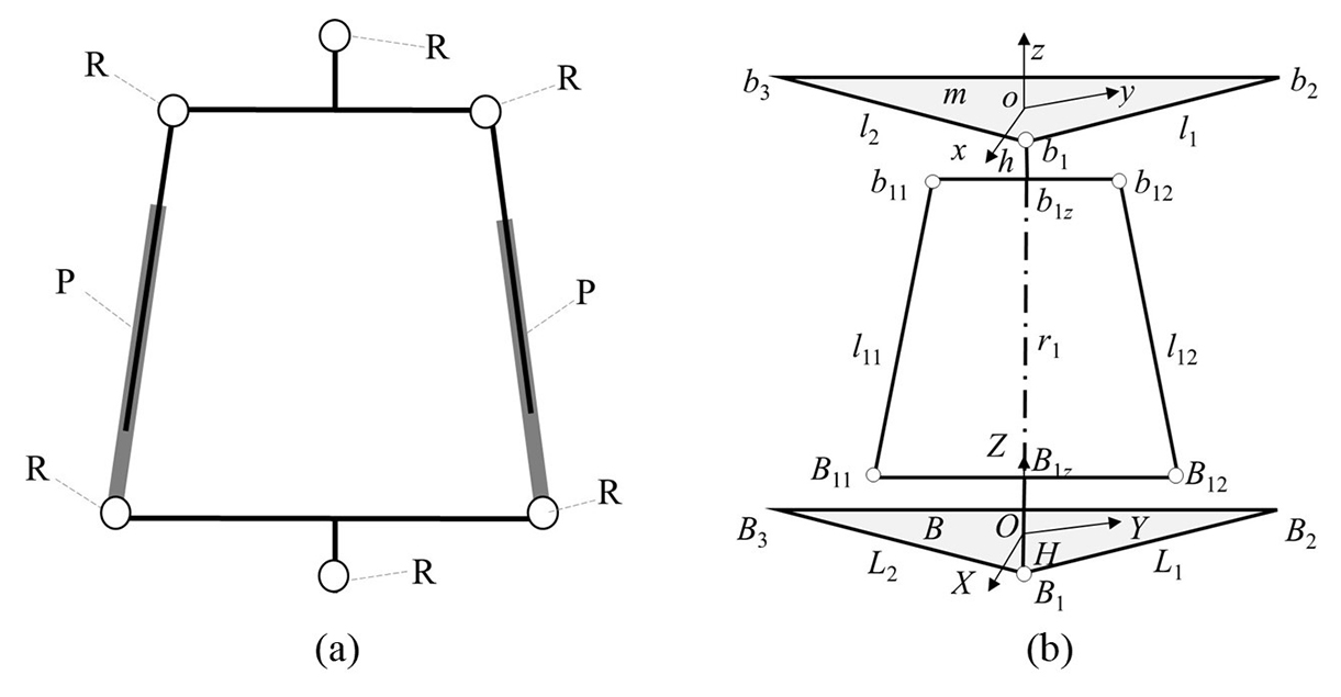
Figure 2 (a) Equivalent six-bar closed loop of elastic bracket; (b) equivalent six-bar closed loop parallel mechanism of sensor.

The mechanism comprises three identical branches that are uniformly distributed along the moving platform. The endpoints of the moving platform, b₁, b₂, and b₃, are connected as equilateral triangles with a side length of l and a center point at o. The three endpoints B₁, B₂, and B₃ of the base B are connected as equilateral triangles with side lengths L and a center point at O. In the moving platform, the base is established on a coordinate system, where the moving coordinate system o–xyz has its origin at o, with the y axis pointing towards endpoint b₂ of the moving platform, the z axis is perpendicular to the moving platform and points upward, and the x axis is established according to the right-hand rule of the coordinate system. The base coordinate system O–XYZ has its origin at O, with the Y axis pointing towards endpoint B₂ of the fixed platform, the Z axis is perpendicular to the plane of the fixed platform and points upward, and the X axis is established according to the right-hand rule of the coordinate system. The vector h, that is b_1Zb₁, is perpendicular to the moving platform and intersects the upper crossbeam at the point b_1Z. The vector H is perpendicular to the base and intersects the lower crossbeam at point B_1Z. The Jacobi matrix (Li et al., 2016) expression for this parallel mechanism is given by

$$\begin{array}{}\text{(1)}& \begin{array}{rl}& {\mathbf{J}}_{\mathrm{h}}={\left(\begin{array}{cc}{\mathit{\delta }}_{\mathrm{ij}}^T& {\left[\left({\widehat{e}}_i-\widehat{\mathit{h}}\right){\mathit{\delta }}_{\mathrm{ij}}\right]}^{\mathrm{T}}\end{array}\right)}_{\mathrm{1}\times \mathrm{6}}+{\left({\widehat{\mathit{e}}}_{\mathrm{ij}}{\mathit{\delta }}_{\mathrm{ij}}\right)}^{\mathrm{T}}\\ & \left({\displaystyle \frac{\left({\mathit{E}}_{\mathrm{3}\times \mathrm{3}}-{\mathit{D}}_{\mathrm{3}}\right)}{{\mathit{D}}_{\mathrm{2}}}}{\mathit{D}}_{\mathrm{0}}\left[{\widehat{\mathit{\delta }}}_i^{\mathrm{2}}-{\widehat{\mathit{\delta }}}_i^{\mathrm{2}}\left({\widehat{\mathit{e}}}_i-\widehat{\mathit{h}}\right)\right]+\left(\begin{array}{cc}{\mathbf{0}}_{\mathrm{3}\times \mathrm{3}}& {\mathit{D}}_{\mathrm{3}}\end{array}\right)\right).\end{array}\end{array}$$

In Eq. (1) δ_i and δ_ij are the unit direction vectors of the virtual branch r_i and the driving branch l_ij, respectively, e_i and e_ij are the distances between b_i and o and b_ij and b_i, respectively, e_i and e_ij are the vectors of the rods b_io and b_ib_ij, respectively ($i=\mathrm{1},\mathrm{2},\mathrm{3}$ $j=\mathrm{1},\mathrm{2}$), and D₀, D₂, and D₃ are vectors related to the angular velocities of the rods.

Based on the principle of virtual work, it can be observed that the sum of the virtual work done by all the driving rods and the virtual work done by the generalized load is zero. The virtual displacement corresponding to the driving force F_l is expressed by the velocity V_l at the corresponding pose, and the virtual displacement corresponding to the loading force at the reference point of the movable platform is expressed by the generalized velocity at the corresponding pose, V, which is given by

$$\begin{array}{}\text{(2)}& {\mathit{F}}_l^{\mathrm{T}}{\mathit{V}}_l=-\left({\mathit{F}}^{\mathrm{T}}{\mathit{T}}^{\mathrm{T}}\right)\mathit{V}.\end{array}$$

It follows that

$$\begin{array}{}\text{(3)}& {\mathbf{J}}_{\mathrm{h}}^{\mathrm{T}}{\mathit{F}}_l=-\left(\begin{array}{c}\mathit{F}\\ \mathit{T}\end{array}\right),{\mathit{F}}_l=-{\left({\mathbf{J}}_{\mathrm{h}}^{-\mathrm{1}}\right)}^{\mathrm{T}}\left(\begin{array}{c}\mathit{F}\\ \mathit{T}\end{array}\right).\end{array}$$

The Jacobi matrix J_h has been derived from Eq. (3). This completes the force mapping from the external loads to the six branches.

Let K_j be the matrix that maps the force from each force-measuring branch to each force-measuring unit, and from the geometry of the bracket, the sensor deformation δv_si is equal to the frame deformation δv_ei, so that

$$\begin{array}{}\text{(4)}& \mathit{\delta }{v}_{\mathrm{si}}=\mathit{\delta }{v}_{\mathrm{ei}}=\mathit{\delta }{v}_i.\end{array}$$

From the conservation of energy, the work done by F_li on the force-measuring branch is equal to the sum of the work done by F_ei acting on the flexible kinematic pairs and F_si acting on the force-measuring unit:

$$\begin{array}{}\text{(5)}& \begin{array}{rl}& F_{\mathrm{li}}\mathit{\delta }{v}_i=F_{\mathrm{ei}}\mathit{\delta }{v}_{\mathrm{ei}}+F_{\mathrm{si}}\mathit{\delta }{v}_{\mathrm{si}},\\ & F_{\mathrm{li}}=F_{\mathrm{ei}}+F_{\mathrm{si}},i=\mathrm{1},\mathrm{2},\mathrm{\dots },\mathrm{6}.\end{array}\end{array}$$

From Eq. (5),

$$\begin{array}{}\text{(6)}& F_{\mathrm{li}}=F_{\mathrm{ei}}+F_{\mathrm{si}}=\left(k_{\mathrm{ei}}+k_{\mathrm{si}}\right)\mathit{\delta }{v}_i={\displaystyle \frac{k_{\mathrm{ei}}+k_{\mathrm{si}}}{k_{\mathrm{si}}}}{F}_{\mathrm{si}},\end{array}$$

where k_ei represents the advective stiffness of the ith flexible kinematic pair, and k_si represents the stiffness of the ith force-measuring unit. Therefore, the 6 × 6 stiffness matrix K_j is

$$\begin{array}{}\text{(7)}& \begin{array}{rl}& {\mathbf{K}}_j=\\ & \left(\begin{array}{ccccc}\left(k_{\mathrm{e}\mathrm{1}}+k_{\mathrm{s}\mathrm{1}}\right)/k_{\mathrm{s}\mathrm{1}}& \mathrm{\cdots }& \mathrm{0}& \mathrm{\cdots }& \mathrm{0}\\ \mathrm{⋮}& \mathrm{\cdots }& \mathrm{⋮}& \mathrm{\cdots }& \mathrm{⋮}\\ \mathrm{0}& \mathrm{0}& \left(k_{\mathrm{ei}}+k_{\mathrm{si}}\right)/k_{\mathrm{si}}& \mathrm{\cdots }& \mathrm{0}\\ \mathrm{⋮}& \mathrm{⋮}& \mathrm{⋮}& \mathrm{⋮}& \mathrm{⋮}\\ \mathrm{0}& \mathrm{\cdots }& \mathrm{0}& \mathrm{0}& \left(k_{\mathrm{e}\mathrm{6}}+k_{\mathrm{s}\mathrm{6}}\right)/k_{\mathrm{s}\mathrm{6}}\end{array}\right).\end{array}\end{array}$$

k_e is the stiffness of the flexible pair consisting of four single-sided straight circular flexible hinges, the expression of which is given in Eq. (4).

To calculate the static mapping array, it is essential to determine the stiffness of the force measurement unit. However, as the internal structure and composition of standard tensile force sensors are not well understood, there is currently no fixed formula for their stiffness. This study employs a combination of theoretical and experimental methods to determine the stiffness of the sensor. By applying pressure F_z in the Z direction on the six-dimensional force sensor loading platform and observing the sensor's indication, the stiffness of the force-measuring unit can be calculated using Eq. (6) as

$$\begin{array}{}\text{(8)}& k_{\mathrm{S}}={\displaystyle \frac{k_e}{\frac{F_{\mathrm{li}}}{F_{\mathrm{si}}}-\mathrm{1}}},k_e={\displaystyle \frac{\mathrm{4}{k}_z}{g^{\mathrm{2}}}}={\displaystyle \frac{Eh{r}^{\mathrm{2}}}{\mathrm{3}{c}_r{g}^{\mathrm{2}}}}.\end{array}$$

From Eq. (6), the six force measurement branches F_li to six force measurement units F_si force mapping can be derived from the stiffness relationship between the two:

$$\begin{array}{}\text{(9)}& \begin{array}{rl}& {\left(\begin{array}{cccccc}{F}_{l\mathrm{1}}& F_{l\mathrm{2}}& F_{l\mathrm{3}}& F_{l\mathrm{4}}& F_{l\mathrm{5}}& F_{l\mathrm{6}}\end{array}\right)}^{\mathrm{T}}\\ & ={\mathbf{K}}_j{\left(\begin{array}{cccccc}{F}_{s\mathrm{1}}& F_{s\mathrm{2}}& F_{s\mathrm{3}}& F_{s\mathrm{4}}& F_{s\mathrm{5}}& F_{s\mathrm{6}}\end{array}\right)}^{\mathrm{T}}.\end{array}\end{array}$$

It follows that

$$\begin{array}{}\text{(10)}& \begin{array}{rl}& \left(\begin{array}{c}\mathit{F}\\ \mathit{T}\end{array}\right)=-{\mathbf{J}}_{\mathrm{h}}^{\mathrm{T}}{\mathit{F}}_{\mathrm{li}}=-{\mathbf{J}}_{\mathrm{h}}^{\mathrm{T}}{\mathbf{K}}_j{\mathit{F}}_{\mathrm{si}},\\ & {\mathit{F}}_{\mathrm{si}}=-{\mathbf{K}}_j^{-\mathrm{1}}{\left({\mathbf{J}}_{\mathrm{h}}^{\mathrm{T}}\right)}^{-\mathrm{1}}\left(\begin{array}{c}\mathit{F}\\ \mathit{T}\end{array}\right)={\mathit{D}}_{\mathrm{1}}\left(\begin{array}{c}\mathit{F}\\ \mathit{T}\end{array}\right).\end{array}\end{array}$$

This completes the static model of the sensor equivalent to the model of the six-bar closed-loop parallel mechanism.

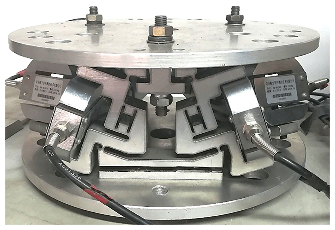
The static model lays the theoretical foundation for the design of the sensor prototype, which is then machined and manufactured. The overall assembly of the sensor is shown in Fig. 3.

Figure 3 Prototype of sensor.

4 Sensor static calibration experiment

Accurate hydrostatic modeling can significantly enhance the ability of sensors to deliver precise force measurements in complex environments. Nevertheless, the performance of a sensor is not solely determined by its structural design and hydrostatic modeling; rather, it is also strongly influenced by its calibration process. Calibration is a crucial phase in optimizing the sensor's performance, ensuring its accurate measurements in real-world applications. Calibration compensation is the most effective approach to enhancing the performance of sensors under existing hardware constraints. The accuracy of calibration has a direct impact on the measurement accuracy of sensors (Yao, 2010). This step is crucial for assessing the actual input–output performance of a sensor.

4.1 Linear static calibration experiment program

Due to the fact that the actual prototype cannot be an absolutely linear system, calibration experiments involve repeated loading and unloading processes in various directions. The loads should encompass the entire range of the sensor, and the average value of the data should be taken to minimize errors caused by system nonlinearity and randomness, thereby enhancing calibration accuracy.

The sensor calibration steps are as follows:

• 1.

  divide the full measurement range into several loading values for each direction;

• 2.

  adjust the calibration device, zero the tool, connect the data cable, and debug the data acquisition system;

• 3.

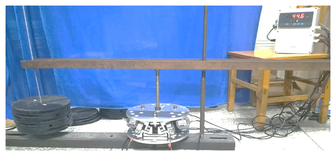
  gradually increase the load to maximum value according to the loading plan in one loading direction, then gradually reduce the load to 0; repeat more than three times, recording the corresponding data (The −F_z direction calibration experiment is shown in Fig. 4.);

• 4.

  follow step 3 for reversed load; repeat more than three times and record the data;

• 5.

  apply loads in the other directions separately according to steps 3 and 4 to complete the data collection for all six load components;

• 6.

  process the collected data, obtain the sensor calibration matrix, and determine indicators such as error matrix, repeatability, and hysteresis.

Figure 4 Calibration experiments for −F_z directions.

4.2 Experimental calibration results and their fitting

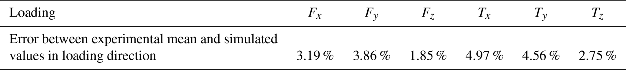
Consider experimental data corresponding to one load case. The measurement results are shown in Fig. 5a; it can be seen that when loading the sensor in the translational z direction, the forces measured by each of the measuring unit were different. Because it was difficult to ensure that the calibration loading point was exactly at the center of the platform, the average value of all force-measuring units can be used, as shown in Fig. 5b. The calibration results are listed in Table 1. It can be seen that the maximum error between the measured average values and the simulated values in each loading direction was 4.97 % in the rotational x direction, and the maximum coupling error generated in the non-loaded direction was 5 %. The results of multiple experiments need to be considered to reduce random errors.

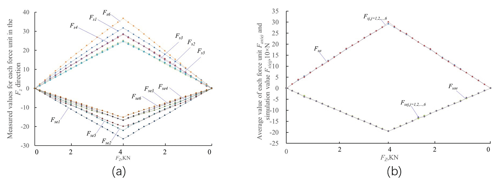
Figure 5 Measured (F_sje) and simulated (F_sj) forces due to incremental loads in z directions. (a) Loading in F_Z direction; (b) load in F_Z direction and takeing the average value.

Table 1 Example of calibration results.

4.3 Nonlinear static calibration of sensors

Calibration experiments allow for the procurement of precise output data from the six-dimensional force sensor under defined load conditions, serving as a pivotal metric for evaluating sensor performance. Nevertheless, to fully realize the potential of these data in achieving high-precision force measurements, it is imperative to address the issue of coupling in the sensor's output signals. The application of decoupling algorithms offers a straightforward and cost-effective solution for this endeavor, representing the primary method of decoupling.

The decoupling of a multi-dimensional force sensor essentially involves establishing a unique least-error input–output relationship for the sensor (Li et al., 2017). However, it is challenging to intuitively determine the relationship between experimental measurements and the input load. Therefore, mathematical methods are required to fit the data, enabling prediction of the output due to an unknown load. Common data fitting methods include end-base, least squares, neural networks, and fuzzy inference (Wu, 2022).

Assuming that the sensor is a linear system, the least squares method can achieve high fitting accuracy (Liu, 2023). However, the six-dimensional force sensor system is generally nonlinear (Yang et al., 2022), and a fitting method that can approximate the nonlinear relationship with high accuracy is required.

Deep learning models, particularly those excelling in handling complex and nonlinear aspects such as artificial neural networks (ANN), one-dimensional convolutional neural networks (1DCNN), long short-term memory (LSTM), bidirectional LSTM (BiLSTM), and attention mechanisms, could potentially provide effective solutions for decoupling the output data from six-dimensional force sensors. These models, through learning and training, can automatically extract useful features from the input data and discover complex mapping relationships between inputs and outputs.

ANN is an ideal tool for decoupling the output data from six-dimensional force sensors due to its unique characteristics, facilitating accurate decoupling and reliable force measurement. Here are the reasons why ANN is suitable for this task:

• 1.

  Parallel processing. The ANN's ability to process information in parallel enables it to efficiently handle the vast amount of data output from six-dimensional force sensors.

• 2.

  Self-learning and adaptability. The ANN can automatically optimize its parameters to adapt to different environments and task requirements, making it resilient to factors such as ambient temperature and sensor aging.

• 3.

  Strong fault tolerance and robustness. In practical applications, the output data from six-dimensional force sensors may be affected by various noises, including mechanical vibrations and temperature drifts. However, ANN can, to a certain extent, ignore these disturbances and extract useful information from the data.

Comparatively, the 1DCNN excels in processing data with significant internal correlations, such as pixel sequences in images or time-series data (Ye and Li, 2022). However, the output data from six-dimensional force sensors typically encompass force and torque information across six distinct dimensions, where the internal local correlation among this information is not prominent. Consequently, in such scenarios, the advantages of the 1DCNN may not be fully realized.

LSTM and BiLSTM networks excel at capturing long-term dependencies in sequential data (Siami-Namini et al., 2019). However, if the output data from a six-dimensional force sensor lack distinct sequential characteristics, meaning that the force and torque information across various dimensions are not closely related sequentially, then these methods may not be the optimal choice.

The application of attention mechanisms in models can assist in automatically learning and focusing on the most relevant parts for decoupling tasks while ignoring unimportant information (Qin and Hu, 2020). However, when dealing with six-dimensional force sensor data, complex cross-interference issues may arise, necessitating stronger feature extraction and representation capabilities. To achieve this, it may be necessary to integrate other nonlinear fitting methods, such as deep neural networks, but such operations may increase model complexity and computational costs.

The neural network method, which defines the input–output relationships of a model by mimicking the structure of neurons in the brain, is a commonly used nonlinear fitting method in engineering (Ma et al., 2019). The neural network method has a powerful self-organizing learning capability (Fan et al., 2019). By using a large amount of linear calibration data as the basis, the artificial neural network method can more accurately predict sensor measurements. The sensor neuron model studied in this paper is shown in Fig. 6.

Figure 6 Neuron model of sensor.

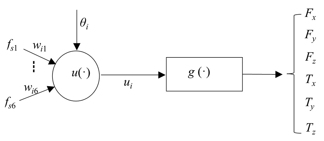
The input–output relationship of the model is

$$\begin{array}{}\text{(11)}& \begin{array}{rl}& u_i=\sum _{j=\mathrm{1}}^{\mathrm{6}}\left(w_{\mathrm{ij}}{f}_{\mathrm{sj}}+{\mathit{\theta }}_i\right),\\ & y_i=g\left(u_i\right)={\left(\begin{array}{cccccc}{F}_x& F_y& F_z& M_x& M_y& M_z\end{array}\right)}^{\mathrm{T}}.\end{array}\end{array}$$

In Eq. (11), f_sj (j= 1, 2, 3, 4, 5, 6) is the input signal of the ith neuron, y_i is the output of the ith neuron, θ_i is the bias value of this neuron, w_ij is the connection weight from cell i to cell j, u(⋅) is the output basis function obtained by superpose of input signals; and g(⋅) is the excitation function of the neuron. The excitation function is taken as an S-type function, which maps the input signal of the neuron onto the interval $(-\mathrm{1},\mathrm{1})$; the function is

$$\begin{array}{}\text{(12)}& g\left(x\right)={\displaystyle \frac{\mathrm{1}-e^{-\mathrm{ax}}}{\mathrm{1}+e^{-\mathrm{ax}}}},\left(-\mathrm{1}<g\left(x\right)<\mathrm{1}\right).\end{array}$$

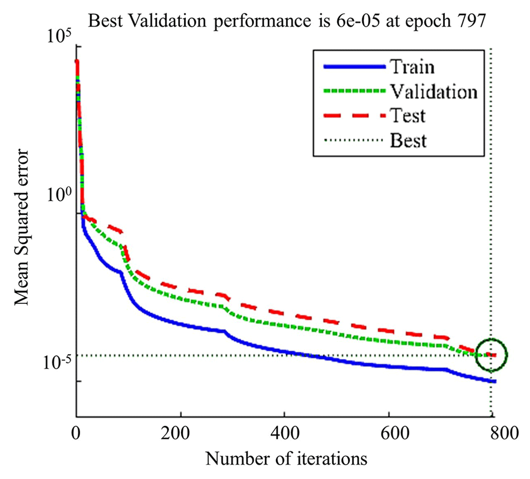
In this study, the LMBP algorithm, a derivative of the backpropagation (BP) algorithm based on the Levenberg–Marquardt (LM) method, is employed as the optimization technique. LMBP integrates the gradient descent method and the Gauss–Newton method within neural networks (Wang et al., 2019), leveraging the advantages of both techniques. This approach not only expedites the training speed of the network but also mitigates the issue of local minima during convergence, thereby enhancing the overall stability of the neural network system. For the purpose of this study, the “trainlm” function available in MATLAB software was utilized for implementing neural network training. The network architecture comprises a total of 10 layers, with the input layer receiving the static linear calibration experimental data obtained from six force measurement units. The output layer generates the six-dimensional force acting on the loading platform. The neural network training results are summarized in Fig. 7, which provides a visual representation of the network's performance.

Figure 7 Results of neural network training.

To ensure accurate calibration, the collected experimental data were used as inputs, and the 194 sets of sample data were divided into three separate groups. The training group, consisting of 70 % of the samples, was utilized to train the neural network and fine-tune its weight parameters based on error feedback. The calibration set, comprising 15 % of the samples, was employed to assess the network's generalization capability. This capability refers to the machine learning algorithm's ability to adapt to novel samples. Networks with robust generalization abilities can also produce accurate outputs for input data that fall outside the learning set. The training process was terminated once the network's generalization ability no longer improved. The remaining 15 % of the samples formed the test group, serving as independent samples to evaluate the quality of the network during and after training.

After 797 iterations, the network's generalization ability attains an optimal state, with the mean square error achieving a magnitude of 10⁻⁵. At this point, all neural network weight values are determined, resulting in a highly accurate nonlinear model for fitting experimental data. When six force measurement unit values are used as inputs, the six-dimensional force outputs obtained via the network closely align with the actual applied six-dimensional forces, with a maximum error of 0.95 % in the loaded direction and a maximum coupling error of 1.33 % in the unloaded direction. It is worth noting that as more sample data are input during training, a higher post-fitting accuracy is achieved.

4.4 LabVIEW-based sensor calibration software

LabVIEW, a graphical programming language (Zang et al., 2023), is a powerful tool that streamlines complex procedures into intuitive flowcharts. Its robust data interface enables seamless integration with various software components. In this study, we integrate the MATLAB-trained neural network into the LabVIEW software to develop a calibration software for the sensor. This software utilizes collected data to establish a direct mapping with the externally applied six-dimensional force, ultimately facilitating nonlinear calibration of the sensor.

The nonlinear calibration software workflow is designed as follows: the collected experimental data signals are converted into a data matrix format. Subsequently, the input data undergo a zeroing process within the software to ensure the accuracy of the test data in the absence of a zero setting. The processed matrix is then fed into the neural network unit. The neural network generates output data that are converted into the six-axis force components, which are then displayed.

The trained neural network module of MATLAB software is called and embedded in the program via a script node, as shown in Fig. 8, and the node outputs the result of the neural network operation.

Figure 8 Calling the neural network module in LabVIEW.

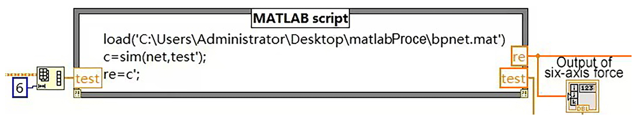
Figure 9 presents the panel of the nonlinear calibration procedure, which illustrates the processed data matrix after the zeroing step, the rows of data to be converted, the values of the six-dimensional force components of the external loads, and the amplitudes of the force measurement unit and the external loads.

Figure 9 Nonlinear static calibration software.

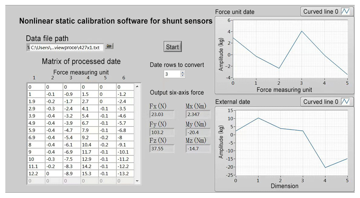
The nonlinear static calibration software offers a visual representation of the sensor loading platform's impact on the external load's component values. Additionally, it enables observation of the force unit's amplitude and external loads, preventing prolonged overload operation of the system. The software features intuitive and straightforward operation, facilitating easy debugging.

5 Sensor applications and their performance enhancement

The decoupling algorithm effectively addresses the coupling interference in the output signal of the sensor, significantly enhancing the accuracy and stability of measurements. This lays the groundwork for the practical implementation of the six-dimensional force sensor. When the robot is stationary or moving at low speed and when the sensor measures the contact force between the end actuator and the environment, the captured data include non-contact forces, such as gravity, along with the actual contact force. This introduces a certain bias in the sensor's readings. To accurately represent the true end force, gravity compensation is necessary. Algorithms are employed to compensate for this, enhancing both the operational performance and adaptability of the parallel robot. This paper proposes a gravity compensation method based on CAD variable geometry to enhance the measurement accuracy of sensors.

Jin et al. (2022) proposed a gravity compensation method that combines active and passive compensation techniques, aiming to enhance the force feedback performance of tactile devices. This method features a simple principle that does not require complex reasoning or calculations, making it easy to implement. However, it is currently only suitable for tactile devices that perform translational movements. When a six-dimensional force sensor is mounted on the wrist of a robot for gravity compensation and the robot typically performs spatial movements, solving for the forward kinematics of the robot's spatial position becomes necessary. In such cases, a gravity compensation method based on CAD variable geometric methods is more suitable for compensating the gravity effects on the six-dimensional force sensor at the wrist of a parallel robot. Zhao et al. (2020) employed multi-body simulation techniques to devise a gravity compensation method for the flexible mesh of a mesh antenna. This approach effectively reduces the discrepancies between ground verification data and on-orbit flight data for mesh antennas, thus ensuring the successful on-orbit operation of satellites. However, when robots perform high-precision tasks such as flexible machining and assembly, their drive modules must adjust their position and attitude based on real-time force information feedback from six-dimensional force sensors. Utilizing CAD variable geometric methods, a wire-frame model can be used to establish a one-to-one correspondence between the physical robot and its wire-frame representation. This allows for real-time and accurate simulation of the forward kinematics of parallel robots, enabling online gravity compensation for six-dimensional force sensors mounted on the robot's wrist. Therefore, this method offers superior advantages in robotic applications such as flexible machining and assembly.

5.1 Gravity compensation algorithms

In the absence of systematic error and without any external environmental contact forces such as human hand force or collision force, the signal generated by the six-dimensional force sensor is solely due to the tool's gravity (Chun, 2022). The orientation of the tool's gravity within the sensor's coordinate system is depicted in Fig. 10.

Figure 10 The direction of the tool's gravity in the sensor coordinate system.

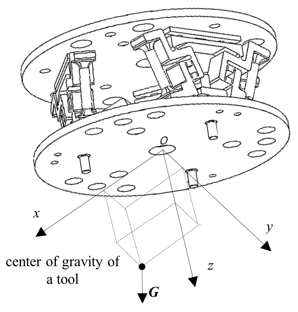
To establish a right-angle coordinate system o–xyz with the center of the sensor loading platform as the origin, the coordinates of the center of gravity of the tool are $(x_G,y_G,z_G)$, and the gravity vector is designated as G. The components of G within the sensor coordinate system can be expressed as ($G_{\mathrm{ox}},G_{\mathrm{oy}},G_{\mathrm{oz}}$). The moment vectors of G relative to the x, y, and z axes are designated as M_Gx, M_Gy, and M_Gz. From the positive direction of each coordinate axis, with the moment counterclockwise to the positive. According to Fig. 11, the following relationships hold for each component of the gravity and moment vectors:

$$\begin{array}{}\text{(13)}& \left\{\begin{array}{l}{M}_{\mathrm{Gx}}=G_{\mathrm{oz}}\times y_G-G_{\mathrm{oy}}\times z_G,\\ M_{\mathrm{Gy}}=G_{\mathrm{ox}}\times z_G-G_{\mathrm{oz}}\times x_G,\\ M_{\mathrm{Gz}}=G_{\mathrm{oy}}\times x_G-G_{\mathrm{ox}}\times y_G.\end{array}\right.\end{array}$$

Equation (13) can be rewritten in matrix form:

$$\begin{array}{}\text{(14)}& \left(\begin{array}{c}{M}_{\mathrm{Gx}}\\ M_{\mathrm{Gy}}\\ M_{\mathrm{Gz}}\end{array}\right)=\left(\begin{array}{ccc}\mathrm{0}& G_{\mathrm{oz}}& -G_{\mathrm{oy}}\\ -G_{\mathrm{oz}}& \mathrm{0}& G_{\mathrm{ox}}\\ G_{\mathrm{oy}}& -G_{\mathrm{ox}}& \mathrm{0}\end{array}\right)\left(\begin{array}{c}{x}_G\\ y_G\\ z_G\end{array}\right).\end{array}$$

M_Gx, M_Gy, and M_Gz in Eq. (14) can be measured by a six-dimensional force sensor.

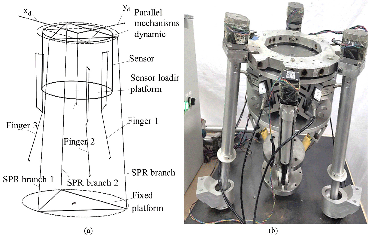
Figure 11 (a) Wire frame of the 3-SPR parallel mechanism. (b) Parallel robot hybrid hand with sensor.

Given that the direction of the tool's gravity, defined by the coordinates of its center of gravity (x_G, y_G, z_G), varies with the pose of the parallel robot, it is essential to establish the relationship between the center of gravity coordinates and the robot's pose. To this end, the developed six-dimensional force sensor was integrated into the wrist of the existing 3-screw-prismatic-revolute (3-SPR) parallel robot, which is used to connect the robot's hand claw with the body and measure the six-dimensional force signal of grasping an object. The robot serves as the executing mechanism, responsible for tasks such as flexible machining and assembly. Meanwhile, the six-dimensional force sensor functions as a feedback mechanism, providing real-time force information that allows the robot to adjust its position and posture dynamically, thereby completing machining tasks with greater precision. Figure 11a and b provide physical drawings of the 3-SPR parallel robot and its structural wire frame with dimensions, respectively and o–x_dy_dz_d is the coordinate system of the movable platform.

The combination structure of the parallel robot is as follows: the base of the six-dimensional force sensor at the wrist is solidly connected to the dynamic platform of the parallel mechanism, and the sensor loading platform is solidly connected to the three single-degree-of-freedom grippers. The bottom of the SPR branch is fixed to a flat steel plate by a strong magnet, and the magnet base is connected to the S joint of the branch. In case of any interference or abnormal rod force, the magnet can be automatically detached from the steel plate, preventing potential damage to the robot's components. The control system incorporates a PC as the main controller, with the motion control card connected to its PCI (Peripheral Component Interconnect) interface. This configuration ensures robust and reliable control. Technical specifications include a maximum torque of 0.88 N m for the branch stepping motor and 0.45 N m for the hand claw stepping motor. The stepping motor driver features a refined control system with 15 subdividing steps and an automatic half-current function, ensuring smooth and precise output currents ranging from 0.64 to 2.14 A. The motor driver interfaces directly with the motion control card, allowing individual control of each motor through distinct interfaces.

From the installation form of the sensor, it can be seen that the sensor coordinate system is in the same direction as the coordinate system of the moving platform of the parallel mechanism. Then the gravity of the tool in the wrist six-dimensional force sensor coordinate system of the projection of the three coordinate axes are

$$\begin{array}{}\text{(15)}& \left\{\begin{array}{l}{G}_{\mathrm{0}x}=G\times \cos {\mathit{\alpha }}_{\mathrm{d}},\\ G_{\mathrm{0}y}=G\times \cos {\mathit{\beta }}_{\mathrm{d}},\\ G_{\mathrm{0}z}=G\times \cos {\mathit{\gamma }}_{\mathrm{d}},\end{array}\right.\end{array}$$

where α_d, β_d, and γ_d are the angles between the tool gravity and the three coordinate axes of the sensor coordinate system, and G_ox, G_oy, and G_oz are the tool gravity components. Substituting Eq. (15) into Eq. (13) yields

$$\begin{array}{}\text{(16)}& \left(\begin{array}{c}{G}_{\mathrm{ox}}\\ G_{\mathrm{oy}}\\ G_{\mathrm{oc}}\\ M_{\mathrm{Gx}}\\ M_{\mathrm{Gy}}\\ M_{\mathrm{Gz}}\end{array}\right)=G\left(\begin{array}{c}\cos {\mathit{\alpha }}_{\mathrm{d}}\\ \cos {\mathit{\beta }}_{\mathrm{d}}\\ \cos {\mathit{\gamma }}_{\mathrm{d}}\\ y_G\cos {\mathit{\gamma }}_{\mathrm{d}}-z_G\cos {\mathit{\beta }}_{\mathrm{d}}\\ z_G\cos {\mathit{\alpha }}_{\mathrm{d}}-x_G\cos {\mathit{\gamma }}_{\mathrm{d}}\\ x_G\cos {\mathit{\beta }}_{\mathrm{d}}-y_G\cos {\mathit{\alpha }}_{\mathrm{d}}\end{array}\right).\end{array}$$

Given the challenges associated with theoretically determining the position positive solution for the 3-SPR mechanism and the real-time angle between gravity and the sensor coordinate system, this study opts to utilize a wire-frame diagram of the mechanism to simulate the positional state of the moving platform in real time. Figure 12 depicts a representative state of the parallel robot during the gripping tool load movement.

Figure 12 Wire-frame simulation of motion process of parallel mechanism.

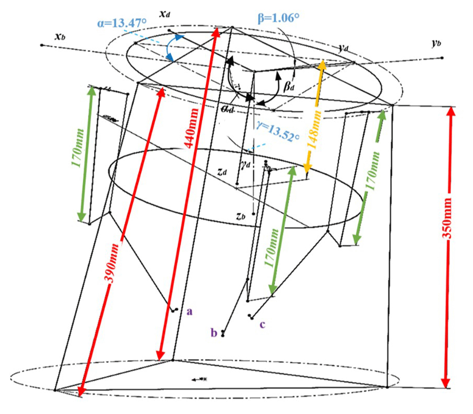
In Fig. 12, different color annotations are used to distinguish various dimensions and parameters. Specifically, green annotations indicate the fixed length of the 3-SPR robot's gripper, which measures 170 mm. Red annotations represent the length of the 3-SPR robot's prismatic pairs at the current pose. Yellow annotations denote the height between the sensor center and the moving platform of the parallel mechanism. Blue annotations depict the Euler angles, which are used to describe the robot's pose information. Black annotations indicate the angles between the tool's gravity and the three axes of the sensor coordinate system. Additionally, points a, b, and c in the figure mark the fingertip sections of the robot's gripper.

Notably, the lengths of the three parallel branches undergo changes, decreasing from the initial 445 to 350, 390, and 440 mm, respectively. Similarly, the lengths of the three hand claw drive rods increase from the initial 137 to 170 mm. The parallel mechanism's moving platform coordinate system is defined by the x_d, y_d, and z_d axes, whereas the base coordinate system of the parallel mechanism consists of the x_b, y_b and z_b axes. The Euler angles α, β, and γ represent the rotation angles between the two coordinate systems. The motion control software acquires real-time angle data based on the dimensional parameters obtained from the wire-frame diagram: α= 13.47°, β= 1.06°, γ= 13.52 °, α_d= 103.47 °, β_d= 91.06 °, γ_d= 13.52°. These values are then inserted into Eq. (16) to determine the tool's gravity component under the sensor system in its pose. To prevent singular matrices from emerging during calculations, the motion control of parallel robots involves selecting N non-coplanar poses and acquiring corresponding six-dimensional force signals to generate N sets of data.

$$\begin{array}{}\text{(17)}& \left(\begin{array}{c}{M}_{\mathrm{Gx}\mathrm{1}}\\ M_{\mathrm{Gy}\mathrm{1}}\\ M_{\mathrm{Gz}\mathrm{1}}\\ M_{\mathrm{Gx}\mathrm{2}}\\ M_{\mathrm{Gy}\mathrm{2}}\\ M_{\mathrm{Gz}\mathrm{2}}\\ \mathrm{⋮}\\ M_{\mathrm{GxN}}\\ M_{\mathrm{GyN}}\\ M_{\mathrm{GzN}}\end{array}\right)=\left(\begin{array}{ccc}\mathrm{0}& G_{\mathrm{oz}\mathrm{1}}& -G_{\mathrm{oy}\mathrm{1}}\\ -G_{\mathrm{oz}\mathrm{1}}& \mathrm{0}& G_{\mathrm{ox}\mathrm{1}}\\ G_{\mathrm{oy}\mathrm{1}}& -G_{\mathrm{ox}\mathrm{1}}& \mathrm{0}\\ \mathrm{0}& G_{\mathrm{oz}\mathrm{2}}& -G_{\mathrm{oy}\mathrm{2}}\\ -G_{\mathrm{oz}\mathrm{2}}& \mathrm{0}& G_{\mathrm{ox}\mathrm{2}}\\ G_{\mathrm{oy}\mathrm{2}}& -G_{\mathrm{ox}\mathrm{2}}& \mathrm{0}\\ \mathrm{⋮}\\ \mathrm{0}& G_{\mathrm{ozN}}& -G_{\mathrm{oyN}}\\ -G_{\mathrm{ozN}}& \mathrm{0}& G_{\mathrm{oxN}}\\ G_{\mathrm{oyN}}& -G_{\mathrm{oxN}}& \mathrm{0}\end{array}\right)\left(\begin{array}{c}{x}_G\\ y_G\\ z_G\end{array}\right)\end{array}$$

To determine the coordinates of the tool's center of gravity in the sensor's coordinate system versus the magnitude of the force of gravity, Eq. (17) is employed, and then the coordinates of the center of gravity in the base coordinate system can be calculated by using the Euler angles α, β, and γ and pose vectors collected from the wire-frame diagram. Let F_ox, F_oy, and F_oz represent the force signals captured by the six-dimensional force sensor. After accounting for gravity compensation, the external force exerted on the six-dimensional force sensor by the external environment can be determined

$$\begin{array}{}\text{(18)}& \left(\begin{array}{c}{F}_{\mathrm{wx}}\\ F_{\mathrm{wy}}\\ F_{\mathrm{wz}}\\ M_{\mathrm{wx}}\\ M_{\mathrm{wy}}\\ M_{\mathrm{wz}}\end{array}\right)=\left(\begin{array}{c}{F}_{\mathrm{ox}}-G_{\mathrm{ox}}\\ F_{\mathrm{oy}}-G_{\mathrm{oy}}\\ F_{\mathrm{oz}}-G_{\mathrm{oz}}\\ M_{\mathrm{ox}}-M_{\mathrm{Gx}}\\ M_{\mathrm{oy}}-M_{\mathrm{Gy}}\\ M_{\mathrm{oz}}-M_{\mathrm{Gz}}\end{array}\right).\end{array}$$

According to Eq. (18), it is evident that the gravity-compensated six-dimensional force sensor signal can accurately reflect the contact force between the gripped tool and the external environment, which provides accurate force feedback information for the active supple control of parallel robots.

5.2 Gravity compensation experiments

In this section, a tool gravity compensation experiment is conducted on the wrist six-dimensional force sensor of the 3-SPR parallel robot. A load is applied to the tool, and the six-dimensional force generated by this load on the sensor in different poses is measured. The parallel robot control system is constructed using a PC and motion control card, and the motion control software interface is presented in Fig. 13a. The software is based on the CAD variable geometry principle and SolidWorks API interface for software secondary development, enabling virtual teaching, motion control, and other functions. The CAD variable geometry method offers a simple, efficient, and practical approach to solving the pose, velocity, and acceleration of a parallel mechanism. Users can quickly solve it without deep background knowledge (Xu, 2010).

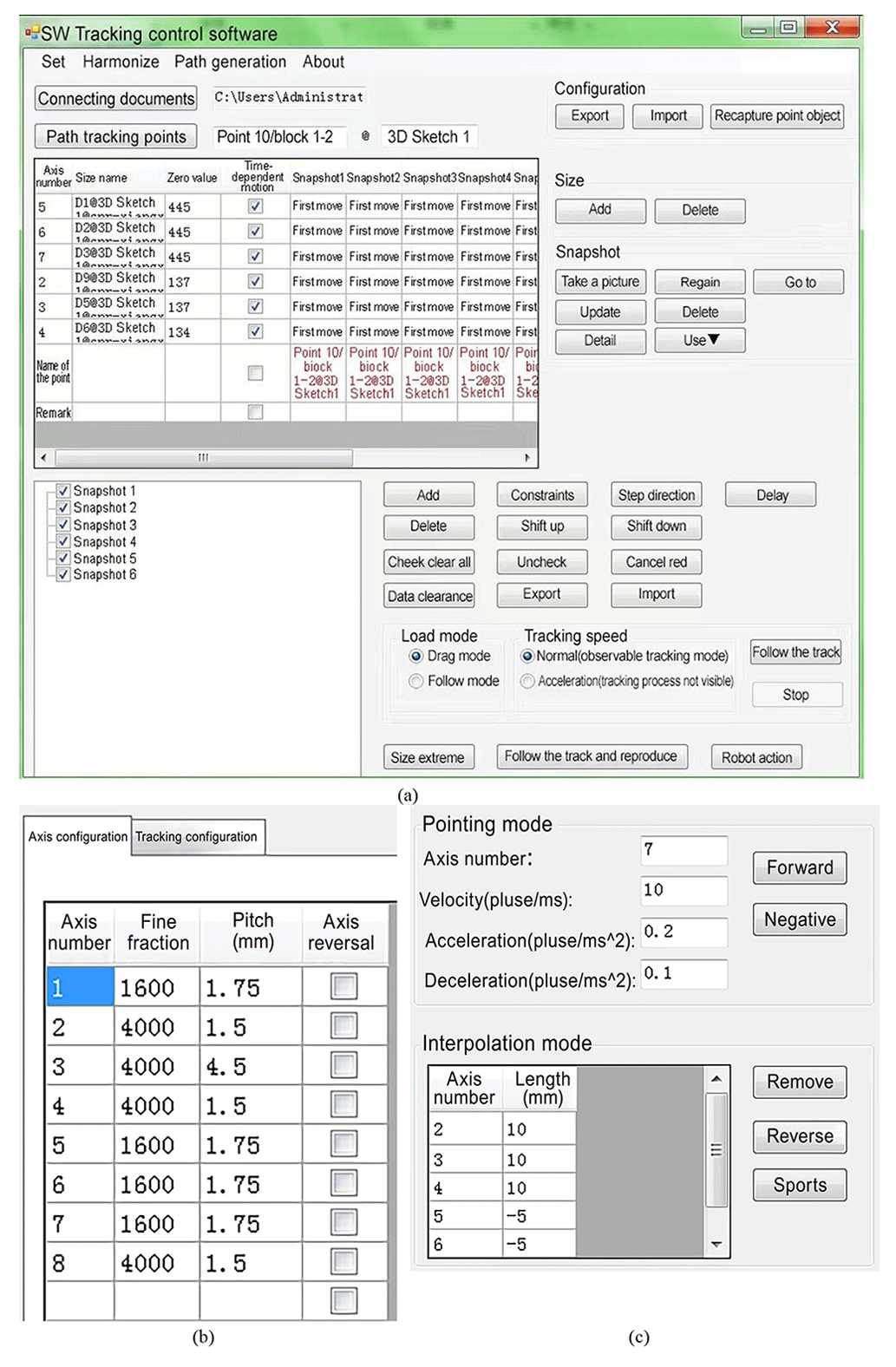
Figure 13 (a) Motion control software of parallel mechanism; (b) motion parameter setting of parallel mechanism.

The experiment is conducted with multiple sets of sampling points to collect six-dimensional forces from the tool to the sensors in various poses of the parallel robots, along with simultaneous robot trajectory planning. Prior to the experiment, the robot requires adjustment and testing. Initially, the motion parameters of the hand claw and leg drive units of the parallel robot are established, as illustrated in Fig. 13b. Axes 2, 3, and 4 represent the robot leg drive units; axes 5, 6, and 7 represent the robot hand claw drive units; and axes 1 and 8 are unoccupied. After entering the appropriate fine fraction and pitch, the zero pose of all drive units is adjusted individually using the pointing mode, with the initial extension of the leg bar set at 445 mm and the initial extension of the hand claw set at 137 mm.

After setting the speed and acceleration of all drive units, the interpolation mode is used to achieve simultaneous movement of one or more drive units to observe whether the program is running normally. It is determined that there is no collision or interference of parts during the planned robot movement. Finally, the robot linkage is initiated for the gravity compensation experiments. The gravity compensation experiment process is presented in Fig. 11b.

The steps of the gravity compensation experiment are as follows:

• 1.

  We collect the six-dimensional force data of the sensor in the no-load state of the parallel robot and check whether the zeroing function of the acquisition software is normal.

• 2.

  The parallel robot hand grips are controlled to grasp the tool and move to the initial pose, and six-dimensional force data are collected.

• 3.

  The parallel robot is controlled to move continuously from the first sampling point and simultaneously collect six-dimensional force data from all set sampling points.

• 4.

  Returning to the initial pose, a heavy load was applied to the tool, and the six-dimensional force generated by the tool weight on the sensor was recorded for different poses.

• 5.

  We return all loads to the ground, release the three hand claws, and return the parallel robot to its initial pose.

Some of the sampling point data and force components collected by the sensors in the experiment are shown in Table 2.

Table 2 Experimental data of partial sampling point.

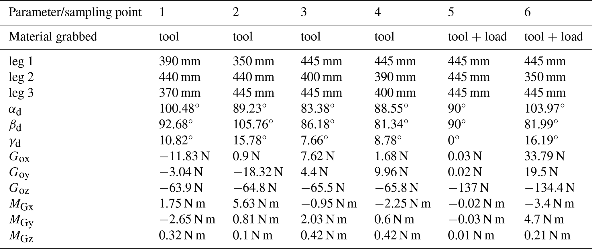
Using Eq. (17) and the data presented in Table 2, we can infer that the tool's average gravity is approximately 66 N. Furthermore, the center of gravity of the tool, when considered within the sensor system's coordinates, is located at [4.73 mm, −8.63 mm, 271 mm]. To determine the coordinates of this center of gravity within the base coordinate system, we utilize the pose transformation matrix between the base and sensor coordinate systems. Once the heavy load is added, the combined weight of the tool and load amounts to 137 N. The gravity exerted by this heavy load alone can be calculated as 137–66 N = 71 N. By applying Eq. (18), we can also determine the six-dimensional force components of this heavy load at a specific attitude, along with the center of gravity of the tool plus load within the sensor system's coordinates. Additionally, to measure the weight of the load, it is placed on a weighing scale, resulting in a reading of 7.05 kg. The measurement error in load gravity after compensation for gravity is then determined:

$$\begin{array}{}\text{(19)}& \mathit{\sigma }={\displaystyle \frac{\mathrm{71}-\mathrm{70.5}}{\mathrm{70.5}}}\times \mathrm{100}\mathit{\%}=\mathrm{0.71}\mathit{\%}.\end{array}$$

In terms of the validation of the coordinate values of the center of gravity of the tool within the sensor coordinate system, the location of the form center of the model can be easily determined due to the regular shape of the chosen tool model for the experiment. Assuming a uniform distribution of material mass within the tool, the center of the form and the center of gravity can be considered co-incident points. The coordinate value of the center of gravity of the tool within the sensor coordinate system can be determined through the use of a wire-frame diagram. The coordinates of the center of gravity of the model are (4.66, −8.51, 272.16 mm), which represents an error of approximately 0.43 % in the z-axis component when compared to the computed value obtained through the gravity compensation algorithm.

The gravity compensation algorithm is effective in terms of reducing the load gravity measurement error and the center of gravity coordinate error. Following gravity compensation, the tool grasped by the parallel robot can accurately sense the six-dimensional force exerted by the external environment on the wrist. Additionally, it is capable of determining the location of the center of gravity of the load, thereby providing a foundation for force-following control.

5.3 Measurement accuracy after replacing the force measurement unit or bracket

To meet the requirements of continuous production in collaborating enterprises, one of the design objectives of the sensor developed in this paper is to facilitate easy installation and disassembly, ensuring good interchangeability of all components. Therefore, commercial standard tensile and compressive force sensors are selected for the force-measuring unit, and the support frame is integrally processed using wire cutting to ensure that even if the sensor or support frame is replaced, a certain level of measurement accuracy can be maintained without the need for secondary calibration.

Therefore, this paper proposes accuracy indicators for the replacement of the support frame and force-measuring unit to assess the interchangeability of sensor components.

An experiment is designed in this paper to test these indicators by grasping the same heavy object through the interchange or replacement of the force measuring unit and support frame. After the components are replaced, the entire sensor is placed on a 3-SPR parallel robot, and three claws are installed on the sensor's loading platform to simulate actual working conditions, as shown in Fig. 14. The claws grasp a sand bucket with an unknown mass, and the parallel robot's driving rods and claws are controlled to maintain the same pose before and after the component replacement to avoid deviation in the loading direction. The readings from the six force measuring units are then recorded, and the theoretical weight of the sand bucket is calculated using a theoretical static force model. The actual weight of the sand bucket is then measured using a standard scale, and the deviation between the two is compared.

Figure 14 Test experiment of replacement accuracy index of force unit or bracket.

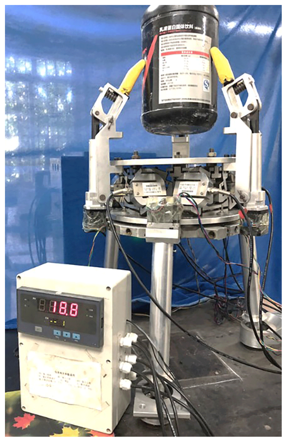
Table 3 Six-dimensional force caused by sand bucket acting on the sensor.

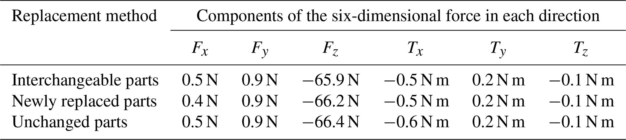
After conducting multiple measurements and averaging the results, the experimental outcomes are summarized in the Table 3. It can be observed from the table that the primary force direction of the sensor is in the F_z direction. Using a standard scale, the mass of the unknown sand bucket is measured to be 6.8 kg. Based on this, it is determined that the measurement error in the F_z direction after interchanging and replacing parts is within 1.2 %. The replacement of the force-measuring unit of the sensor can be quickly put into use without the need for secondary calibration, thus saving time for on-site calibration. Improving the machining precision of the bracket can enhance the accuracy of replacing the sensor bracket and force-measuring unit.

6 Conclusions

In light of the sensor structure's unique characteristics, a method is proposed for modeling the sensor's static force as an equivalent parallel mechanism sensor containing a six-bar closed-loop parallel mechanism.

Sensor static calibration experiments were conducted, and the deviation between the experimental values obtained from a single loading experiment and the simulated values was within 5 %. The artificial neural network approach was employed to fit multiple sets of experimental data, revealing a satisfactory decoupling effect.

A gravity compensation method for the six-dimensional force sensor of the wrist of a robot is proposed based on the CAD variable geometry method. To demonstrate its effectiveness, 3-SPR-type parallel robot hybrid wrist six-dimensional sensor gravity compensation experiments were conducted. The experimental results indicate that the gravity compensation method enables the sensor to more accurately perceive the six-dimensional force of the external load on the operating tool, with load gravity and gravity coordinate values within 1 % error. The objective of our research is to devise six-dimensional force sensors that possess robust applicability and outstanding performance characteristics. To achieve this, further endeavors are requisite in the following areas. In the static calibration experiment of the six-dimensional force sensor, the manual adjustment of the weight masses for each set of data calibration significantly hinders calibration efficiency. Consequently, the current calibration device exhibits a low level of automation, necessitating further design iterations and enhancements.