A replaceable-component method to construct single-degree-of-freedom multi-mode planar mechanisms with up to eight links

The multi-mode planar mechanisms (MMPMs) are excellent-performance reconfigurable mechanisms, which not only inherit structural characteristics of planar mechanisms but also have the multi-task, multi-working-condition application advantages of multi-mode mechanisms. However, lacking common bifurcation analysis and construction methods, their industrial application and development are seriously hindered. This paper presents a replaceable-component method to construct a set of single-degree-of-freedom (single-DOF) MMPMs based on the branch graphs of the corresponding planar mechanisms and the proposed multi-mode modules (MMMs). First, according to the established loop equations, all the kinematic information of the original planar mechanism is obtained by the branch graphs and singularity points using Maple. Then, compared to the relationship between the concepts of the branch and motion mode, the number and continuity of branches are taken as the index to identify the potential bifurcation and mode conversion ability for the corresponding planar mechanisms. Subsequently, the MMM is presented to help the planar mechanisms break the singularity positions to form the corresponding MMPMs, and the steps of constructing single-DOF MMPMs are summarized. Finally, a single-DOF Stephenson six-bar three-mode planar mechanism, a Watt six-bar three-mode planar mechanism, and an eight-bar four-mode planar mechanism are constructed for the first time, and the corresponding multi-mode motion analyses are made. The results can give the available configuration for the design of corresponding MMPMs. The proposed method will provide strong guidance for the configuration design of MMPMs.

1 Introduction

The multi-mode mechanism (Zlatanov et al., 2002a) is an important branch of reconfigurable mechanisms. Compared to other types of reconfigurable mechanisms, it can achieve multi-mode motion by changing its structure without disassembly and assembly. And since no auxiliary devices are required in the conversion process of this kind of mechanism, it has the advantage of rapid mode conversion (Yu et al., 2020), which meets the performance requirements of multiple functions and multiple working conditions for equipment. Therefore, the multi-mode mechanism has attracted great attention from scholars and has become the research hotspot of current mechanism research. The research results have been widely used in innovative designs of high-end mechanical equipment such as in aviation equipment (Agogino et al., 2018; Li et al., 2018), medical rehabilitation (Tseng et al., 2017; Nurahmi et al., 2019; Carbonari et al., 2014), and machining (Azulay et al., 2014; Rico et al., 1999; Wu et al., 2017).

The traditional single-degree-of-freedom (single-DOF) planar mechanism is the mechanism with the lowest degree of freedom among planar mechanisms. It has the advantages of convenient installation, low cost, relatively simple motion trajectory, and convenient control. Due to these characteristics, it is normally the first choice for mechanical equipment design. Despite having been studied for hundreds of years, many scholars are still interested in it. By introducing the mixed-poses concept, Zhao et al. (2021) presented a new synthesis method for single-DOF six-bar linkages, and, based on the results, they successfully designed and tested a rehabilitation device with more accurate motion trajectory for multi-joint coordinated training of human limbs. Lee et al. (2021) provided a quantitative approach to determining the relative performances of single-DOF four-, six-, and eight-bar robotic gait trainers from the standpoint of kinematics, which helps determine cost-effective training solutions for rehabilitation clinics and possibly even for home use. Zhang et al. (2022) proposed the design method for the single-DOF planar-linkage bionic mechanism to solve the problems caused by the multiple variables of the six- or eight-bar mechanisms and the complicated constraint conditions. Liu and Chang (2018) used the so-called Virtual Cam–Hexagon Method to obtain all the instant centers of the planar single-DOF kinematically indeterminate linkages up to 10 bars. The applicable rate of this method is 73 %. Based on instant centers and the rewritten D'Alembert principle, Di Gregorio (2022) proposed geometric and analytic techniques for modeling and studying the dynamic behavior of planar single-DOF mechanisms. The resulting dynamic model is novel and general. Nie et al. (2019) utilized graph theory and transmission angle to locate the dead-center positions of single-DOF planar mechanisms. The dead-center positions of the single-DOF 10-bar and 12-bar planar linkages are first solved. Desai et al. (2019) presented a new single-DOF crank-driven walking-leg mechanism for walking machines and walking robots. It has the characteristics of compact structure, low cost, and high speed, which can be advantageous in industries, agriculture, recreation, autonomous vehicles, and so on.

Based on the above discussion, it has been proven that the traditional single-DOF planar mechanism holds significant application and research value. However, due to the continuous progress of science and technology, as well as the ongoing scarcity of resources and consequent environmental concerns, traditional single-DOF planar mechanisms are unable to meet the demands of current mechanical equipment or mechanisms that require multitasking, multiple working conditions, and various scenes. Therefore, the single-DOF multi-mode planar mechanism (MMPM) is proposed to overcome the limitations of traditional mechanisms. By altering the constraints of singular configuration, the single-DOF MMPM can achieve multi-mode motion and offer both the structural advantages of traditional planar mechanisms and the application benefits of multi-mode mechanisms. This provides a new research direction for single-DOF mechanisms and expands their potential applications. Based on a planar four-bar mechanism, Huang et al. (2023) firstly designed a set of single- and double-stage mechanisms depending on the rule of the degrees-of-freedom formulation; then, the single- and multi-loop reconfigurable platforms are both presented using the above results. Wu et al. (2019) redesigned a three-RRR (rotation joint) spherical parallel manipulator (SPM) of co-axis input with reconfigurability, which can be used directly for the applications such as flight simulators. By utilizing a simple four-bar linkage, the SPM can change virtually the dimensions of driving links. Lin et al. (2022) proposed a concept of the reconfiguration parallel mechanism based on friction self-locking composite joints, which can transform between a truss and a mechanism. In their paper, a parallelogram linkage with two wedge blocks is taken as the JSLTr (JSLT – translation self-locking joint – and JSLR – revolution self-locking joint) of the family of friction self-locking composite joints. Tian et al. (2018) presented a method for configuration synthesis of metamorphic mechanisms based on functional analyses and developed eight source-metamorphic mechanisms, which are obtained by integrating two corresponding planar mechanisms. Wu et al. (2021a, 2023) proposed two types of robots with four working modes for spraying work. By utilizing the four-bar mechanism with two sliders (2021) and the five-bar mechanism (2023) of these two spraying robots, a larger workspace can be achieved. Based on the analysis of three kinds of kinematotropic four-bar mechanisms, Zhang et al. (2022) presented the idea of constructing reconfigurable generalized parallel mechanisms (GPMs) by integrating closed-loop kinematotropic linkages with configurable platforms. Using the proposed method, a 5-degree-of-freedom reconfigurable GPM with the configurable platform is formed and discussed. Wu et al. (2021b) designed a novel dual degree-of-freedom octopod platform with a reconfigurable trunk. To adjust the posture and enlarge the working space of legged modules to enhance the obstacle-climbing capability, the trunk mechanism can be reconfigured into a steering four-bar linkage in steering motion with the aid of the singular feature. Liu et al. (2020) put forward a new reconfigurable multi-mode walking–rolling robot based on the single-loop closed-chain four-bar mechanism, which has four types of motion modes: four-bar walking, four-bar rolling, self-deforming, and six-bar rolling modes. And the robot can be changed to different modes according to the terrain.

Although the single-DOF MMPM has incomparable application advantages compared with the traditional single-DOF planar mechanisms, its research and development are still in the initial stages. This is because of the unique flat structure of the planar mechanism, which makes it difficult to effectively analyze its bifurcation motion and mode conversion. Bifurcation motion and mode conversion motion are the two main motion characteristics of multi-mode mechanisms, which are also the key to forming the corresponding multi-mode mechanism. Bifurcation motion represents the fact that the mechanism can realize multiple motion modes (Dai et al., 2021; Müller, 2014; Hervé, 1999; Angeles, 2004; Wei and Dai, 2020; Zlatanov et al., 2002b), while mode conversion is the means or method by which a mechanism switches from one motion mode to another (Galletti and Fanghella, 2001; Husty and Zsombor-Murray, 1994; Larochelle and Venkataramanujam, 2013; Venkataramanujam and Larochelle, 2014). Generally speaking, bifurcation motion is a prerequisite for mode conversion motion, and only when the mechanism can realize bifurcation motion does it have the possibility of mode conversion motion. In other words, the mechanism must have two or more motion modes before it can perform the corresponding mode conversion operation. Therefore, bifurcation motion is the first problem to be solved in the construction of a multi-mode mechanism. Normally, single-DOF MMPM is established based on the structure of a single-DOF planar mechanism. However, for a single-DOF planar mechanism, there generally exists only one explicit motion mode when the joints are assembled, and it is difficult to reveal the motion mode hidden in the mechanism structure because of the lack of the corresponding identification method (Yu et al., 2020). As a result, designing single-DOF MMPMs often relies solely on researchers' inspirations and experiences, and few structures of single-DOF MMPMs can be formed for application. The development is hindered.

To solve the development dilemma of single-DOF MMPMs, this paper proposes a common method to analyze the potential bifurcation motion of single-DOF planar mechanisms and provides a systematic way to construct the corresponding single-DOF MMPMs. The proposed method may present a new design thought for the configuration design of the MMPMs. Based on loop equations, the corresponding branch graphs and singularity points are obtained to analyze the potential of bifurcation motions of planar mechanisms. Then, according to the mode conversion principle of breaking the singularity positions, the telescopic link-type module (II) is presented and discussed in the multi-mode four-bar planar mechanisms. Subsequently, the steps for constructing single-DOF MMPMs are summarized. Finally, two single-DOF six-bar MMPMs (Stephenson and Watt) and a single-DOF eight-bar MMPM are presented and discussed in this paper for the first time. These new mechanism designs offer numerous potential applications and opportunities for the development of single-DOF MMPMs.

One contribution of this paper is to provide a new method for identifying bifurcation motion, mode conversion, and constructing mechanism configurations of single-DOF MMPMs. The proposed method not only reveals the mechanism of bifurcation movement but also provides design guidance at the structural scale. Furthermore, since the proposed method is based on the loop equations, branch graphs, and the multi-mode modules (MMMs) (all three are common to single-DOF planar mechanisms), it is universally applicable. Additionally, the proposed method provides a graphical insight into the relationship between the configuration formation and the bifurcation motion of the mechanism and presents a new research idea for the study of single-DOF MMPMs. Another contribution is to summarize the corresponding construction steps and to form a single-DOF four-bar MMPM, two single-DOF six-bar MMPMs (Stephenson and Watt), and a single-DOF eight-bar MMPM. To our best knowledge, these last three MMPMs are built for the first time. Simultaneously, multi-mode motion analyses are conducted correspondingly. The results can provide the available configuration for designing corresponding MMPMs and some design guidance.

This paper is organized as follows: in Sect. 2, the basic concepts such as loop equation, branch graph, singularity point, motion mode, motion state, and MMMs are introduced. In Sect. 3, firstly, the number of breaches is taken as an index to identify the bifurcation ability of planar mechanisms. Then, MMMs are used as a tool to implement mode conversion of the MMPMs. Finally, the steps for constructing single-DOF MMPMs are summarized, and the corresponding flow chart is drawn. In addition, multi-mode motion analysis is presented, and the single-DOF four-bar MMPM is taken as an example for explanation. The Stephenson six-bar three-mode planar mechanism, the Watt six-bar three-mode planar mechanism, and the eight-bar four-mode planar mechanism are constructed, and the corresponding multi-mode motion analyses are discussed in Sect. 4. Conclusions are presented at the end of this paper.

2 Basic concepts

2.1 Loop equation

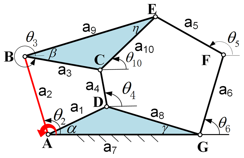
With the digitalization of mechanism configuration, the loop equations can provide all the kinematic characteristic information of the planar mechanism, including link connections, input–output relationships, transient motion, and more. These findings have been proven in Ting and Dou (1996), Ting (1994), Ting et al. (2010), Dou and Ting (1996), Wang et al. (2010), and Nie et al. (2020). Taking the four-bar planar mechanism (Fig. 1) – for example, when the input joint is at the joint A (i.e., the input angle is θ₂), – the following loop equations are established.

Figure 1 Kinematic graph of a four-bar planar mechanism.

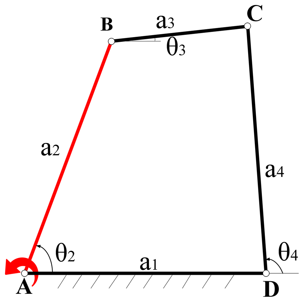
First, we have loop ABCD:

$$\begin{array}{}\text{(1)}& a_{\mathrm{2}}{e}^{i{\mathit{\theta }}_{\mathrm{2}}}+a_{\mathrm{3}}{e}^{i{\mathit{\theta }}_{\mathrm{3}}}-a_{\mathrm{1}}-a_{\mathrm{4}}{e}^{i{\mathit{\theta }}_{\mathrm{4}}}=\mathrm{0}.\end{array}$$

Equation (1) can be written as the following two equations based on Euler's formula:

$$\begin{array}{}\text{(2)}& a_{\mathrm{4}}\cos {\mathit{\theta }}_{\mathrm{4}}-a_{\mathrm{2}}\cos {\mathit{\theta }}_{\mathrm{2}}-a_{\mathrm{3}}\cos {\mathit{\theta }}_{\mathrm{3}}+a_{\mathrm{1}}=\mathrm{0},\end{array}$$

$$\begin{array}{}\text{(3)}& a_{\mathrm{4}}\sin {\mathit{\theta }}_{\mathrm{4}}-a_{\mathrm{2}}\sin {\mathit{\theta }}_{\mathrm{2}}-a_{\mathrm{3}}\sin {\mathit{\theta }}_{\mathrm{3}}=\mathrm{0}.\end{array}$$

Eliminating θ₃, Eq. (1) can be expressed as follows:

$$\begin{array}{}\text{(4)}& \begin{array}{rl}{a}_{\mathrm{1}}^{\mathrm{2}}& +a_{\mathrm{2}}^{\mathrm{2}}-a_{\mathrm{3}}^{\mathrm{2}}+a_{\mathrm{4}}^{\mathrm{2}}-\mathrm{2}{a}_{\mathrm{2}}{a}_{\mathrm{4}}\cos ({\mathit{\theta }}_{\mathrm{4}}-{\mathit{\theta }}_{\mathrm{2}})-\mathrm{2}{a}_{\mathrm{1}}{a}_{\mathrm{2}}\cos {\mathit{\theta }}_{\mathrm{2}}\\ & +\mathrm{2}{a}_{\mathrm{1}}{a}_{\mathrm{4}}\cos {\mathit{\theta }}_{\mathrm{4}}=\mathrm{0}.\end{array}\end{array}$$

Equation (4) is the equation of the one-to-one correspondence between the input joint angle θ₂ and the output joint angle θ₄.

2.2 Branch graph and singularity point

Branches (or circuits) (Nie et al., 2016) are a fundamental issue in the realm of mobility for planar mechanisms. A branch is a gathering of mechanism configurations, referring to the continuous motion of the mechanism. Branches are determined by the link size of the loops and are independent from input conditions (Ting, 1994; Nie et al., 2016). Typically, mechanism configurations of the planar mechanism cannot transform from one branch to another without disconnecting the mechanism. The branch graph is a map containing all the kinematic information of the mechanism. It can be obtained by the loop equations and the concept of joint space rotation (JRS) (Ting, 1994; Ting et al., 2010) and can be drawn in Maple. For the four-bar planar mechanism, whose link parameters are provided in Table 1, a branch graph is shown in Fig. 2 based on Eq. (4). The corresponding singularity points are listed in Table 2. Considering Fig. 2, the red curves are the joint rotation space of the four-bar loop ABCD. There are the two branches (I and II), and each branch has two sub-branches, for example, sub-branch 1-2 and sub-branch 2-1 are the two sub-branches in branch I. Similarly, sub-branch 3-4 and sub-branch 4-3 exist in branch II. Obviously, the two branches and the sub-branches have been separated into singularity points of 1 and 2 and 3 and 4. Furthermore, the two sub-branches cannot occur at the same time in the same branch since the mechanism has only a pair of θ₂, θ₄ at an instantaneous configuration. For example, if the mechanism is in sub-branch 1-2 of branch I (such as instantaneous configuration A), the other sub-branch 2-1 (instantaneous configuration B) does not exist. Normally, the branches of the planar mechanisms cannot be transformed into each other unless the joint is disassembled and re-equipped. But if the planar mechanism has been changed into the corresponding multi-mode mechanism using the following proposed method, the multi-mode mechanism will be able to transform from sub-branch 1-2 to one of the sub-branches 3-4 or 4-3 through the singularity points 2 and 3 (path I) or from sub-branch 2-1 to one of the sub-branches 3-4 or 4-3 through the singularity points 1 and 4 (path II) at one time. Note that path I and path II are only used for purposes of indication and are not specific movement routes. Based on the above discussion, sub-branch 1-2 and sub-branch 2-1 cannot appear simultaneously. Therefore, the transformation of sub-branch 1-2 to sub-branch 2-1 is meaningless. For that reason, in the following part of this paper, no distinction is made between branches and the sub-branches. Besides, the configurations of the four-bar planar mechanism corresponding to each sub-branch in Fig. 2 are shown in Fig. 3. And except for branches and singularity points, the rest of the branch graph (Fig. 2) is the non-branching area, in which the planar mechanism cannot be assembled. The singularity point (Ting,1994; Ting et al., 2010) represents the singular configurations of the mechanism. In these configurations, the mechanism may lose control momentarily and has zero mechanical advantage. Considering Figs. 2 and 3, the singularity points 1, 2, 3, and 4 belong to the forward singularities (the case in which the passive links are collinear, i.e., dead-center position), separating the sub-branches and branches, and there are also four inverse singularities, that is, the inverse singularity points ①, ②, ③, and ④ in Fig. 3 (the case in which the input link is collinear with the link to which it is connected shown). These only affect the motion range of the mechanism and do not change the motion performance of the mechanism as they only involve the input link. Compared to the forward singularities, the inverse singularities have relatively little impact on the mechanism. Therefore, in this paper, singularity positions usually refer to the forward singularities. Last but not least, for the four-bar planar mechanism at the forward singularity point (such as, the forward singularity point 2 in Fig. 3a), the mechanism will degenerate into a stable three-bar mechanism by losing 1 degree of freedom as the input continues to rotate, as shown in Fig. 3a (red arrow). As for the uncertainty of the mechanism at the forward singularity point, this happens when the input of the mechanism changes because there are sub-branches in the same branch of the mechanism. The forward singularity point is the dividing point of the sub-branches of the mechanism; thus, the probability of the mechanism at the forward singularity position choosing which sub-branch to enter is random. For example, in Fig. 2, there are the two sub-branches, 2-1 and 1-2, in branch I. When the input of the mechanism at the forward singularity point 2 changes – that is, changing from the red arrow into the purple arrow – the mechanism will randomly enter sub-branch 1-2 (Fig. 3a) or sub-branch 2-1 (Fig. 3b). However, in this paper, the later discussed mode conversion is mostly based on the condition that the input of the mechanism is unchanged, that is, the degraded degree of freedom mechanism (such as the stable three-bar mechanism case). More importantly, even if the input of the mechanism changes when it is at the forward singularity position, the mechanism randomly enters the sub-branch, but whether the mechanism is converted from sub-branch 1-2 or sub-branch 2-1 to other branches of the mechanism, it will not affect the mode conversion result of the mechanism (see Figs. 3a, b, and 4); thus, the uncertainty of the mechanism at the forward singularity point does not affect the multi-mode mechanism construction method proposed in this paper. In short, according to the discussion above, it is easy to see that the branches are separated by the forward singularity positions.

Table 1 Parameters of the four-bar planar mechanism in Fig. 1.

Figure 2 Branch graph of the four-bar planar mechanism.

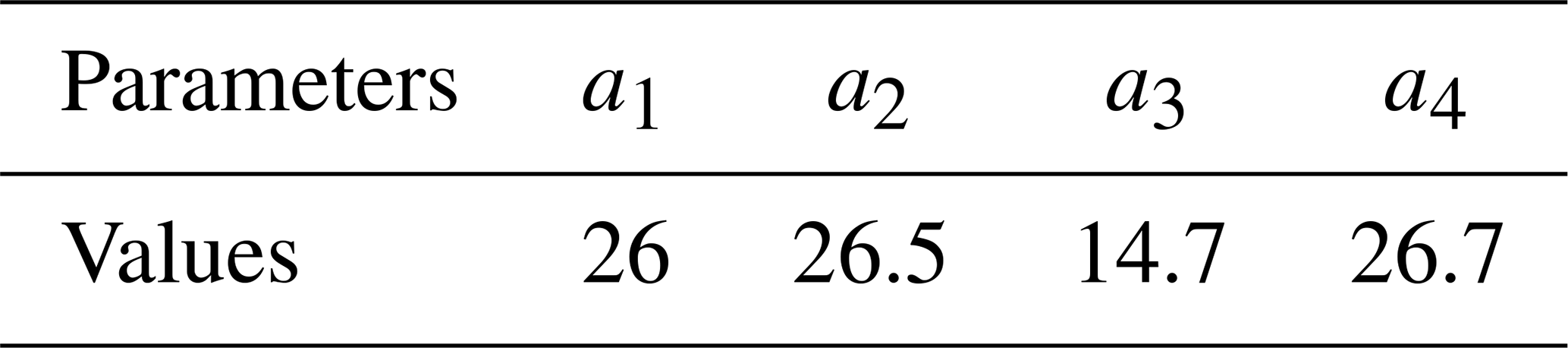
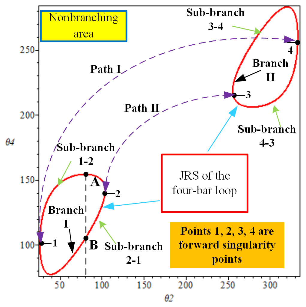
Table 2 Singularity points the four-bar planar mechanism in Fig. 1.

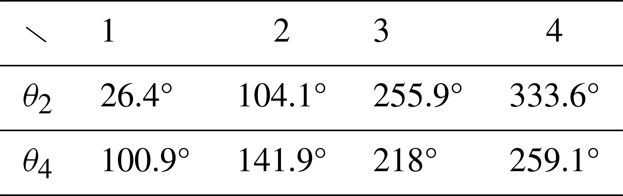
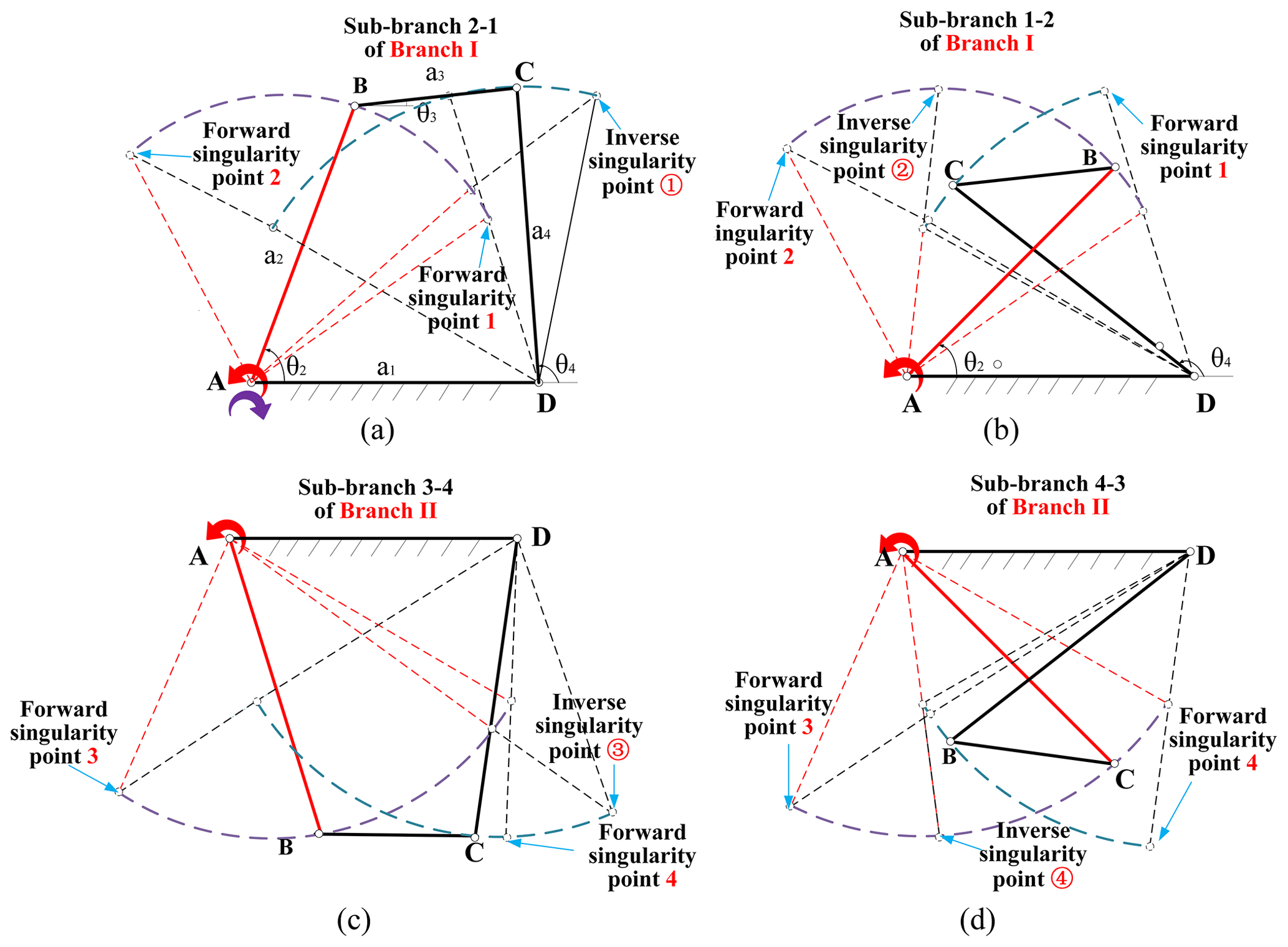
Figure 3 (a) Configuration corresponding to sub-branch 2-1 in Fig. 2. (b) Configuration corresponding to sub-branch 1-2 in Fig. 2. (c) Configuration corresponding to sub-branch 3-4 in Fig. 2. (d) Configuration corresponding to sub-branch 4-3 in Fig. 2. See Table 1 for the parameters of the four-bar planar mechanism in Fig. 1.

2.3 Motion mode and motion state

2.3.1 Motion mode

In this paper, for the planar mechanisms discussed, motion modes are defined as a set of continuous sequences of instantaneous configurations. They are normally separated by singular configurations, and all of them add up to the configuration space of the mechanism. Considering the above definition, motion modes have the following three features: (1) in a motion mode, the mechanism cannot meet any singularity position; (2) any two motion modes are separated by the singular configurations of the mechanism, and the link parameters of the mechanism in different motion modes must be the same; (3) different motion modes result in distinct workspaces, which together make up the configuration space. Comparing the above three features with the discussion about branches in Sect. 2.2, it is easy to see that the concept of motion mode is similar to that of a branch. Actually, in this paper, the branch of the mechanism is equal to its motion mode, and the branch graph, which contains all the branches of the mechanism, is exactly its configuration space. Here, we take the four-bar planar mechanism in sub-branch 2-1 (Fig. 3) and the four-bar planar mechanism in sub-branch 3-4 (Fig. 3) as the examples for explanation in Fig. 4.

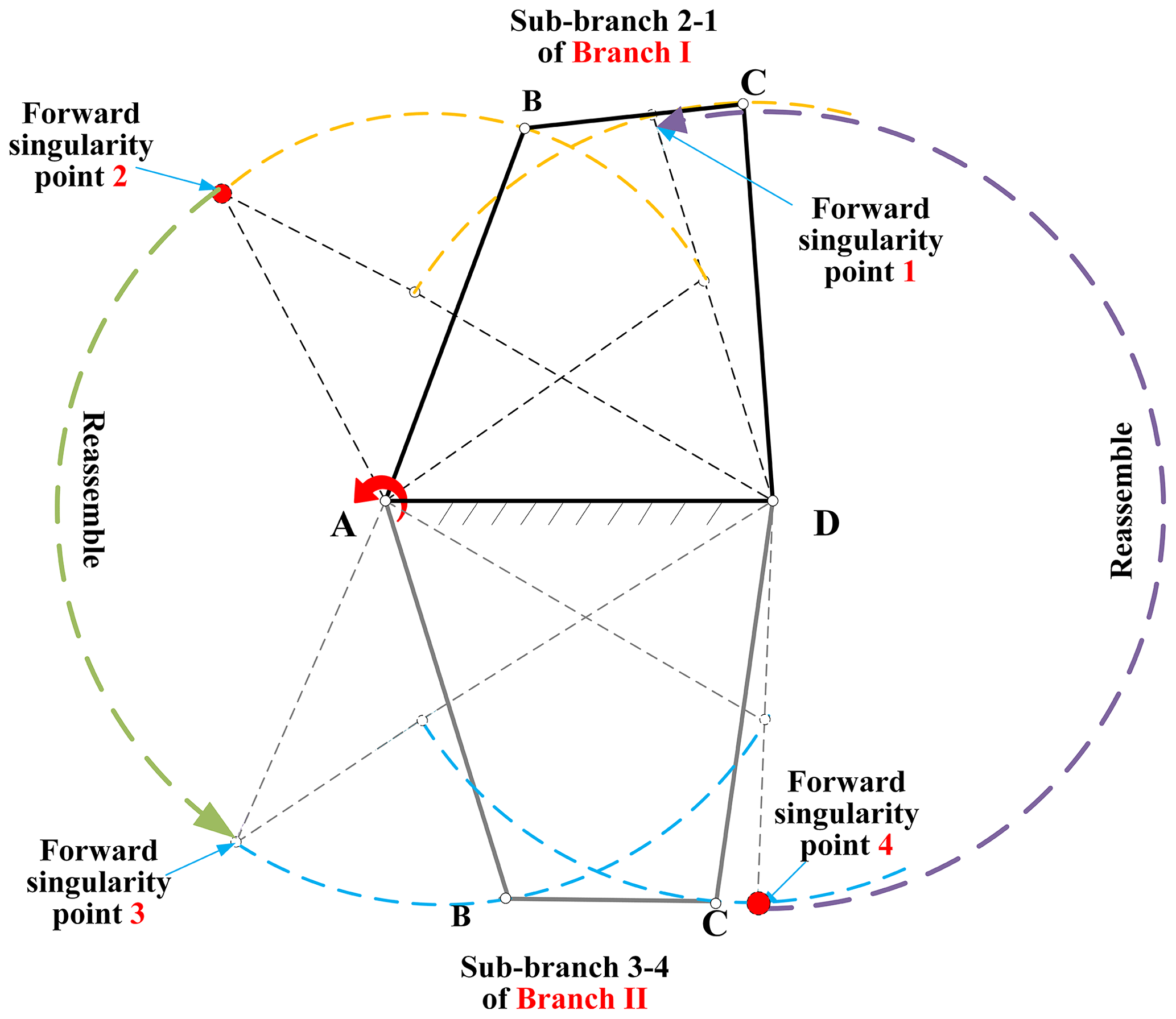
Figure 4 Motion modes of the four-bar planar mechanism in sub-branch 2-1 and in sub-branch 3-4 and the corresponding transition of the two motion modes.

For a certain assembled planar mechanism, the links are limited by the joints, resulting in only one explicit motion mode existing at any given time. Therefore, the four-bar planar mechanism in sub-branch 2-1 has one motion mode, which is represented by the yellow curve when link AB serves as the input. The four-bar planar mechanism in sub-branch 3-4 has another motion mode, i.e., the blue curve, shown in Fig. 4. However, since the two mechanisms have the same parameters and a connected relation in terms of the links, according to loop equations and the definition of branches, they have the same branch graph. This means that they have the same configuration space. Based on the three features of motion modes, to some extent, they can be identified as two motion modes of the same mechanism. Furthermore, the two motion modes just exactly correspond to two branches in the branch graph of the mechanism shown in Fig. 2; i.e., sub-branch 2-1 corresponds to branch I, and sub-branch 3-4 corresponds to branch II. Considering Fig. 2, the two branches are separated by singularity points; the mechanisms in different branches cannot be directly transformed into each other unless the joint (the red one; i.e., the mechanism meets its singular configuration) is disassembled and re-equipped. The purple arrow and green arrow indicate the path of the transition of two motion modes. The green arrow represents branch I to branch II. The purple arrow represents branch II to branch I.

2.3.2 Motion state

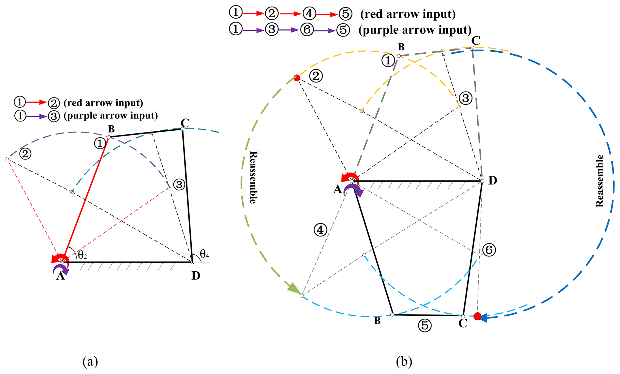
Motion state is used to describe the motions of the mechanisms. It can describe not only the instantaneous motion but also the continuous motion of the mechanism. Different motion states can be distinguished by the changes in motion characteristics (normally, meeting singularity positions) or the link parameters. Compared to motion mode, the mechanism described by motion station can change its link parameters, but the mechanism described by motion mode does not. For a certain planar mechanism, the link parameters in different motion modes must be the same. According to the discussion above, we know that the four-bar planar mechanism (Fig. 1) has a branch graph and two motion modes shown in Figs. 2 and 3a and c. Furthermore, in the motion mode as shown in Fig. 5a, there exist three kinds of motion states: configuration ① (the beginning state, 26.4° $<{\mathit{\theta }}_{\mathrm{2}}<$ 104.1°), configuration ② (the singular state, i.e., singularity point 2, θ₂= 104.1°), and configuration ③ (the singular state, i.e., singularity point 1, θ₂= 26.4°). In the motion mode shown in Fig. 5b, there are three motion states: configuration ④ (the singular state, i.e., singularity point 3, θ₂= 255.9°), configuration ⑤ (the state, 255.9° $<{\mathit{\theta }}_{\mathrm{2}}<$ 333.6°), and configuration ⑥ (the singular state, i.e., singularity point 4, θ₂= 333.6°); these are in addition to configuration ①, configuration ②, and configuration ③. The green arrow and blue arrow (Fig. 5b) indicate the mode state path that the mechanism encounters in turn during the mode transition.

Figure 5 (a) A four-bar planar mechanism. (b) Another four-bar planar mechanism.

2.4 Multi-mode modules

Multi-mode modules (MMMs) are the units that can change their scale or torque under a certain condition. For planar mechanisms, they are commonly used to help the mechanism break the constraint singularity configuration to realize the motion mode transformation (i.e., mode conversion). In our other paper (Nie et al., 2024), depending on how the constraint singularity configuration is changed, MMMs are simply classified into three types (that is, variable-scale module, variable-torque module, and combination module) and are all discussed in detail in single-DOF four-bar MMPMs. Since this paper focuses on the construction method of single-DOF MMPMs, MMMs are only a part of the construction process. Therefore, in the following section of this paper, the telescopic link-type module (II), which belongs to the variable-scale module, is just used as an example to construct the corresponding single-DOF MMPMs. In other words, single-DOF MMPMs containing other multi-mode modules will not be studied in depth.

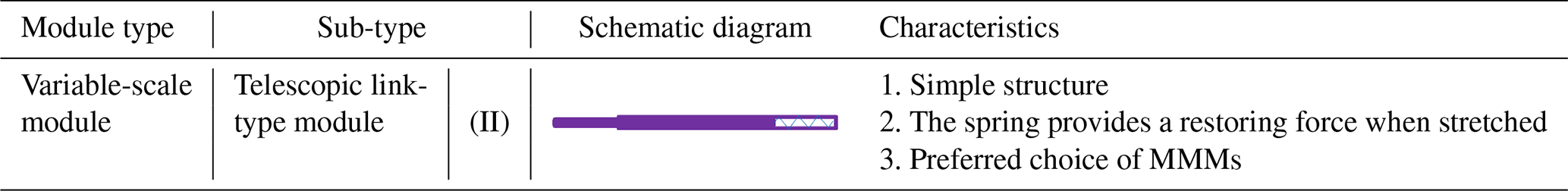
The telescopic link-type module (II) is a component resembling a piston, which is composed of an inside link, a rigid sleeve (note that there is a trapezoid-like cavity in this sleeve, which requires the module to be pulled by more than a certain amount before it can be deformed), and a spring. It can change its link length by pulling the inside link while the spring provides a restoring force accordingly. Based on the simple structure, it has the advantages of low cost and reliable movement, making it the preferred choice of MMMs. However, its disadvantage is the spring in the sleeve, which can cause problems during installation and reduce service life. The schematic diagram and characteristics are listed in Table 3.

Table 3 Schematic diagram and characteristics of the telescopic link-type module (II).

3 Construction method and multi-mode motion analysis

3.1 Identification of bifurcation ability

Bifurcation motion of multi-mode mechanisms indicates that the mechanism can realize multiple motion modes, which is the first issue to be considered. For single-DOF MMPMs, since they are normally established based on the corresponding planar mechanisms, the potential bifurcation ability of these planar mechanisms should be identified first. However, limited by the flat structures, planar mechanisms commonly exhibit only one explicit motion mode, and identifying the remaining motion modes is difficult due to a lack of identification methods. Nevertheless, in this paper, as demonstrated in the above discussion, the meaning of a branch in a branch graph is equivalent to its motion mode. Therefore, the number of breaches serves as an index for identifying the bifurcation ability of planar mechanisms. In other words, if a planar mechanism has two or more branches in its branch graph, it has the potential for bifurcation motion. For example, the branches shown in Fig. 2 illustrate this case. If there are no such branches, then the planar mechanism cannot undergo bifurcation motion. Additionally, the branch graph is influenced by the link parameters of the loop equations of the planar mechanism; therefore, only certain scales of planar mechanisms have potential for bifurcation ability.

3.2 Implementation of mode conversion

Mode conversion is the means or method by which a mechanism switches from one motion mode to another. It is the second main motion characteristic of the multi-mode mechanism. In this paper, we utilize the above-mentioned MMMs to achieve mode conversion and to form corresponding single-DOF MMPMs. For planar mechanisms, the process of implementing mode conversion is as follows. Firstly, after satisfying the bifurcation ability of planar mechanisms, the singularity points (forward singularities) should be located by solving the loop equations. Then, the continuity of the two branches near the singularity point will be checked. If the range of the abscissa or ordinates of two branches near the singularity points increases unidirectionally, the two branches are continuous. For example, in Fig. 2, the singularity points are at points 2 and 3, the two branches are branch I and II, and the abscissa values between branch I (26.4° $<{\mathit{\theta }}_{\mathrm{2}}<$ 104.3°) and branch II (255.9° $<{\mathit{\theta }}_{\mathrm{2}}<$ 333.6°) are unidirectionally increasing. Therefore, the two branches (branch I and II) are continuous. Finally, some links in the mechanism are replaced by the MMMs, usually the driven link closest to the input link, such as the case in Fig. 7. By changing the scale or torque of the MMMs, the mechanism can overcome constraint singularity configurations and achieve mode conversion. What is worth noting is that the number of MMMs to be replaced is not as much as possible but should be selected according to the different requirements of the production needs for the mechanism mode so as to form the structural configuration with the best cost and function. Last but not least, since the mode conversion process only takes place in the non-branching area (such as the case in Fig. 7) in this paper, it means that the scale of the mechanism structure is unchanged (i.e., the loop equations, which affect the kinematic characteristics of the mechanism discussed in Sect. 2.1, are the same) in different motion modes. In other words, the replacement of multi-mode modules hardly affects the mechanism movement in their respective modes.

3.3 Process of constructing a single-degree-of-freedom multi-mode planar mechanism

As mentioned previously, MMPMs are generally based on the structural configuration of traditional planar mechanisms, and the main difference between MMPMs and traditional planar mechanisms lies in bifurcation motion and mode conversion. Therefore, the key to constructing MMPMs is to enable traditional planar mechanisms to exhibit these two motion characteristics. In this paper, for traditional planar mechanisms, (1) to obtain bifurcation ability, the corresponding loop equation and branch graph are established and used to determine whether the traditional planar mechanisms can be transformed into the corresponding MMPMs. If there are at least two branches in the branch graph, then it is possible for the planar mechanisms to become MMPMs. (2) To obtain mode conversion ability, firstly, the singular points of traditional planar mechanisms are identified by the loop equations. Then, the particular links or components suitable for replacement are located when the mechanisms are at the singular configuration. Finally, based on given requirements for motion modes, appropriate MMMs are chosen and replaced to construct MMPMs.

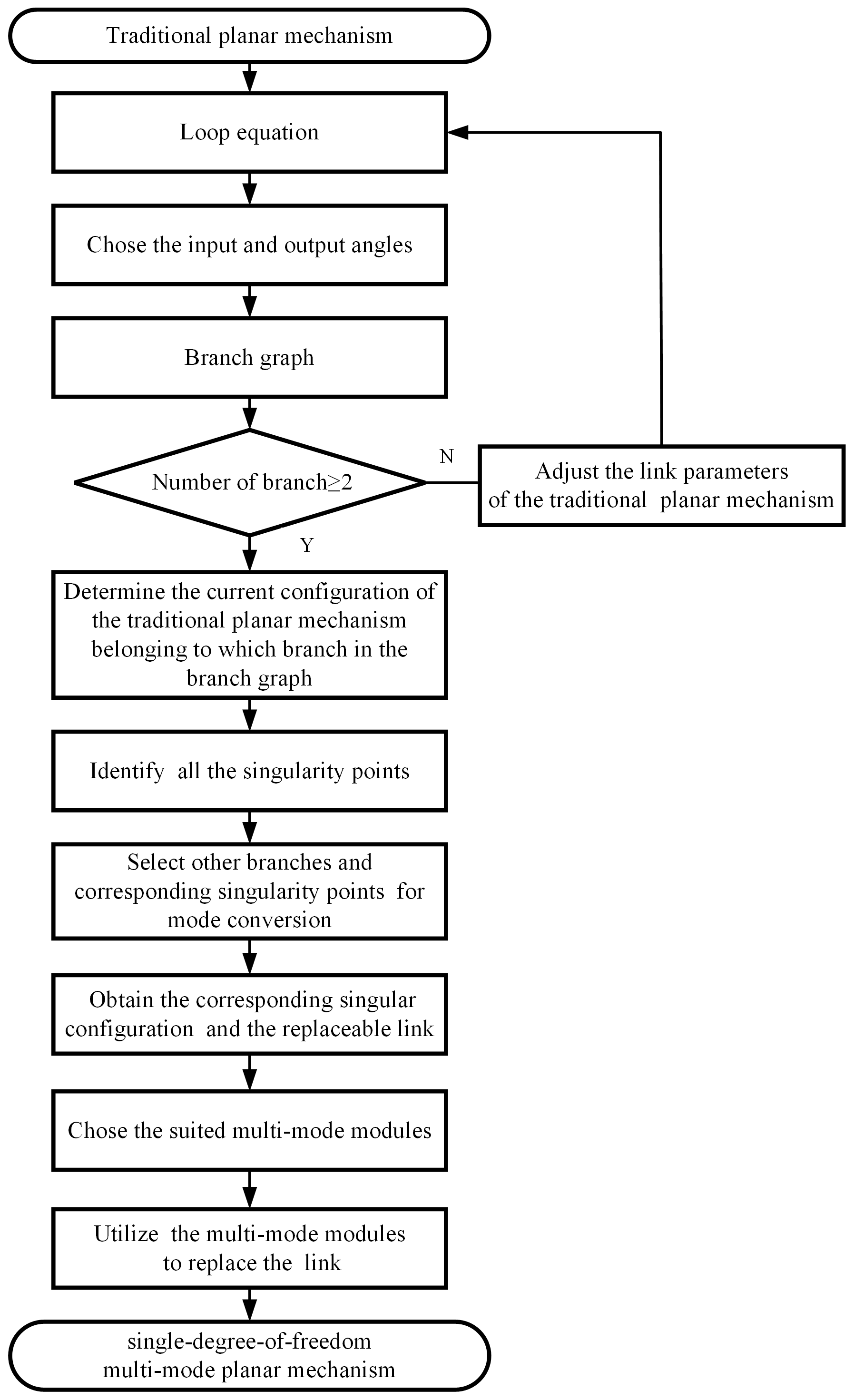
To facilitate understanding, the following steps are summarized, and the four-bar planar mechanism shown in Fig. 1 is used as an example for a detailed explanation. The flow chart for constructing single-DOF MMPMs is shown in Fig. 6.

1. Establish the loop equation of the traditional planar mechanism. After that, choose the input and output angles and obtain the equation of the one-to-one correspondence between the input joint angle and the output joint angle. Subsequently, based on the concept of joint rotation space, draw the corresponding branch graph with Maple. For the four-bar planar mechanism in Fig. 1, the loop equation is Eq. (1); the branch graph is shown in Fig. 2.

2. Check whether the planar mechanisms can be transformed into the corresponding MMPMs based on the number of branches in the branch graph. If the number of branches ≥ 2 (i.e., the case in Fig. 2 for the four-bar planar mechanism), go to step (3). Otherwise, adjust the link parameters in the above loop equation until there exist at least two branches, and then go to step (3).

3. Determine the current configuration of the traditional planar mechanism belonging to a particular branch in the branch graph according to the input range. Then, identify all the singularity points by solving the loop equations. For the four-bar planar mechanism in Fig. 1, all the singularity points are listed in Table 2. The current configuration of the four-bar planar mechanism (Fig. 1) corresponds to branch I in Fig. 2.

4. Select the corresponding other branches and right singularity points for mode conversion based on the requirement of the mechanism function and the number of motion modes. This step is generally considered to be key in determining the excellent performance of the finally constructed MMPMs. However, since this problem involves the performance of the mechanism and is very complicated with many factors, this paper aims to put forward the construction method; thus, it will not be discussed in depth in this paper. As far as mode conversion is concerned in this paper, all branches are involved and not just some branches for convenience. For the four-bar planar mechanism in Fig. 1, since there only two branches in the branch graph, the other branch can only be branch II, and the corresponding singularity point can only be point 2; the input direction is shown in Fig. 1.

5. Based on step (4), obtain the corresponding singular configuration of the mechanism and identify the suitable replacement link or component. For the four-bar planar mechanism in Fig. 1, the singular configuration is the motion state configuration ②, and the replacement link is link BC.

6. Choose the appropriate MMMs and perform the replacement operation to construct the corresponding MMPMs based on motion modes and input conditions. For the four-bar planar mechanism in Fig. 1, the resulting four-bar MMPMs with the proposed method are shown in Fig. 7 and discussed in Sect. 3.4.

Figure 6 Flow chart for constructing four-bar multi-mode planar mechanisms.

3.4 Multi-mode motion analysis

Multi-mode motion analysis mainly involves analyzing motion modes of single-DOF MMPMs and the transformation process between motion modes. Based on the multi-mode mechanism construction method described in Sect. 3.3, the motion mode of the mechanism has been identified based on the loop equations and branch graphs. Therefore, in the following part of this paper, the mode motion analysis mainly refers to how the mechanism realizes the transformation between multiple motion modes. Still taking the four-bar planar mechanism in Fig. 1 as our example, when the mechanism is operated according to Sect. 3.3, the corresponding single-DOF four-bar MMPM with the telescopic link-type module II is shown in Fig. 7a. Based on the definition of motion mode and motion state, there exist two motion modes (i.e., branch I and branch II). Although each motion mode has two sub-branches – that is, there exist four combinations – only two sub-branches can appear at the same time. The detailed explanation can be found in Sect. 2.2. These four combinations are similar for multi-mode motion analysis; therefore, this section will only consider sub-branch 2-1 and sub-branch 3-4. Furthermore, there exist at least nine motion states (Fig. 7a): configurations ①, ②, ③, ④, ⑤, ⑥, ⑦, ⑧, and ⑨. Configuration ① represents the continuous-motion state within the input limit range of branch I. Configuration ② represents the motion state at the input limit position of branch I (the forward singularity point 2, red arrow input). Configuration ③ represents the motion state at the input limit position of branch I (the forward singularity point 1, purple arrow input). Configuration ⑦ represents the motion state in the non-branching area with an increasing scale. At this time, the length of the MMM is the local maximum. Configuration ④ represents the motion state at the input limit position of branch II (the forward singularity point 3, purple arrow input). Configuration ⑤ represents the motion state within the input limit position of branch II. Configuration ⑥ represents the motion state at the input limit position of branch II (the forward singularity point 4, red arrow input). Configurations ⑧ and ⑨ represent the motion state in the non-branching area with an increasing scale. Note that they are the motion states which have the maximum scale in the non-branching area. Configuration ⑧ corresponds to the red arrow input, and configuration ⑨ corresponds to the purple arrow input. As the four-bar MMPM only has two motion modes, there are only two types of mode transitions, namely, (1) branch I to branch II and (2) branch II to branch I, as shown in Fig. 7a, according to different input conditions. For simplicity, the case with the red arrow input is discussed in the following.

Figure 7 Multi-mode motion analysis of single-DOF four-bar MMPMs.

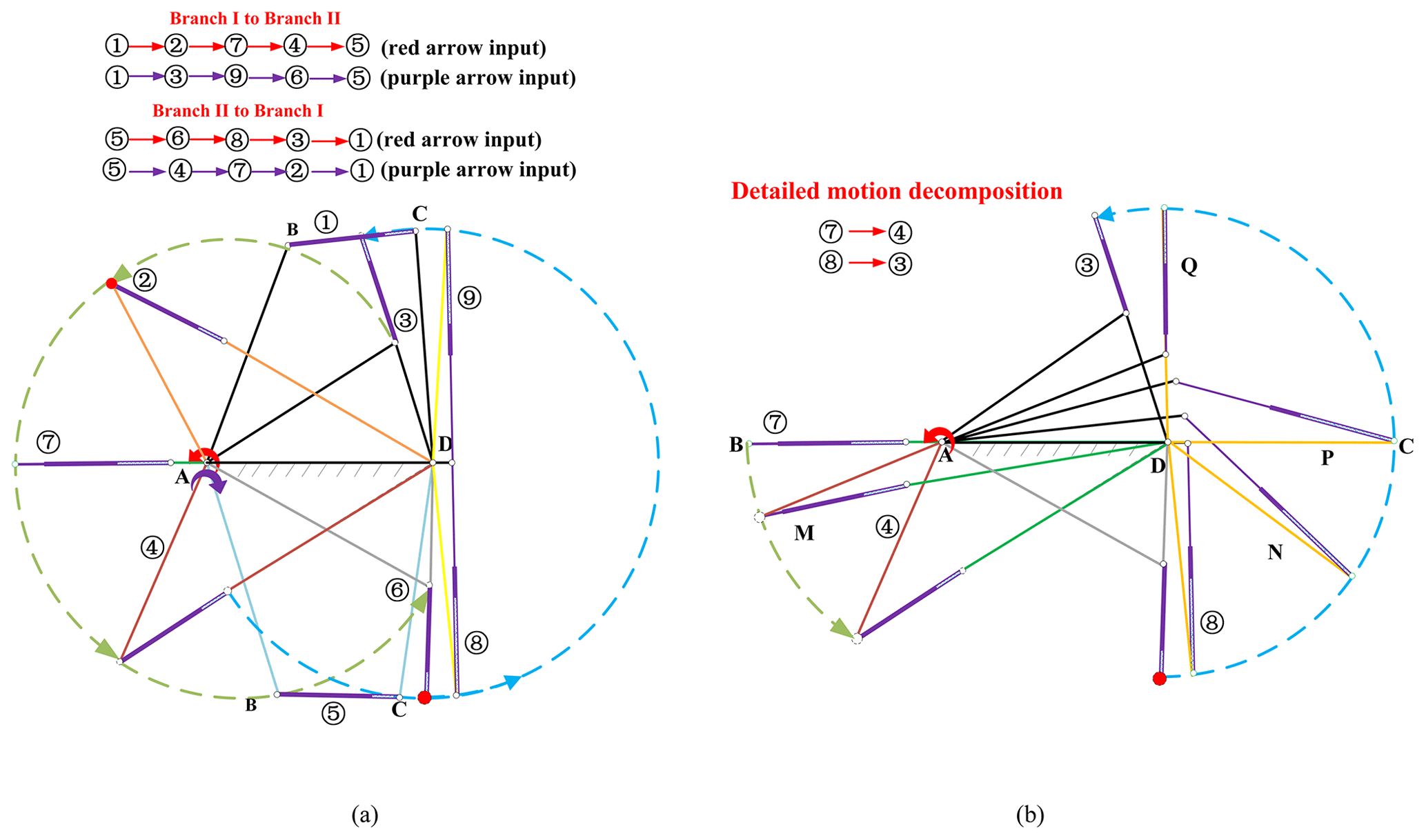
(1) Branch I to branch II. When the four-bar MMPM is switched from branch I to branch II, configurations ①, ②, ⑦, ④, and ⑤ are involved, and the input direction is the red arrow in Fig. 7. The detailed motion decomposition is as follows. In the motion states of configuration ① and configuration ②, the length of the telescopic link-type module (II) is the same as the original size of link BC (Fig. 1). At this time, the four-bar MMPM is in branch I. In the process of configuration ② transforming to configurations ⑦, ④, and ⑤, the telescopic link-type module (II) is in the variable-scale stretching state, and the length of the telescopic link-type module (II) becomes the local longest one in configuration ⑦. In the process of configuration ⑦ transforming to configuration ④, the telescopic link-type module (II) will first go through the local longest stretch, and then it is gradually compressed (configuration M in Fig. 7b) until it reaches the original size (configuration ④ in Fig. 7b) under the spring force of the MMM. Finally, the mechanism will stay in branch II (configuration ⑤ in Fig. 7a).

(2) Branch II to branch I. After successfully transforming the four-bar MMPM from branch I to branch II, as the input link continues to rotate, the MMPM can be directly converted back to branch I by going through configurations ⑥, ⑧, and ③. The detailed motion decomposition of transforming from branch II to branch I is as follows. In the motion states of configuration ⑤ and configuration ⑥, the length of the telescopic link-type module (II) is the same as the original size of link BC (Fig. 1), and the four-bar MMPM is still in Branch II. In the process of configuration ⑥ transforming to configuration ①, the telescopic link-type module (II) is in the variable-scale stretching state, and the length of the telescopic link-type module (II) becomes the longest one in configuration ⑧. At this time, the link AB is horizontally coincident with the link AD, and the longest MMM length a₃ is equal to a₄; in other words, $a_{\mathrm{3}}\ge a_{\mathrm{4}}>a_{\mathrm{2}}>a_{\mathrm{1}}$. Based on the N-bar rotation theorem (Ting and Liu, 1991; Nie et al., 2022), the link AD is the shortest link, and the link AB and the link CD can be the cranks. Furthermore, the MMMs are still the maximum length in configurations N and P (where the link CD is horizontal) in Fig. 7b, and after configuration P, the telescopic link-type module (II) will go through the longest stretch, and then it is gradually compressed (configuration Q in Fig. 7b) until it reaches the original size (configuration ③ in Fig. 7a) with the help of the restoring force provided by the spring in this module. Finally, the mechanism will stay in branch I.

4 Single-degree-of-freedom multi-mode planar mechanisms with up to eight links

4.1 Single-degree-of-freedom six-bar three-mode planar mechanisms

Single-DOF six-bar planar mechanisms are common in the design of mechanical equipment, except for the single-DOF four-bar planar mechanism. In this paper, in order to prove the effectiveness of the proposed method, a Stephenson six-bar planar mechanism (Fig. 8) and a Watt six-bar planar mechanism (Fig. 11) are used as the component basis to construct the corresponding multi-mode mechanisms; see the Stephenson six-bar three-mode planar mechanism shown in Fig. 10 and the Watt six-bar three-mode planar mechanism in Fig. 13.

Figure 8 Kinematic graph of the Stephenson six-bar planar mechanism.

4.1.1 Single-degree-of-freedom Stephenson six-bar three-mode planar mechanism

1. Loop equation established

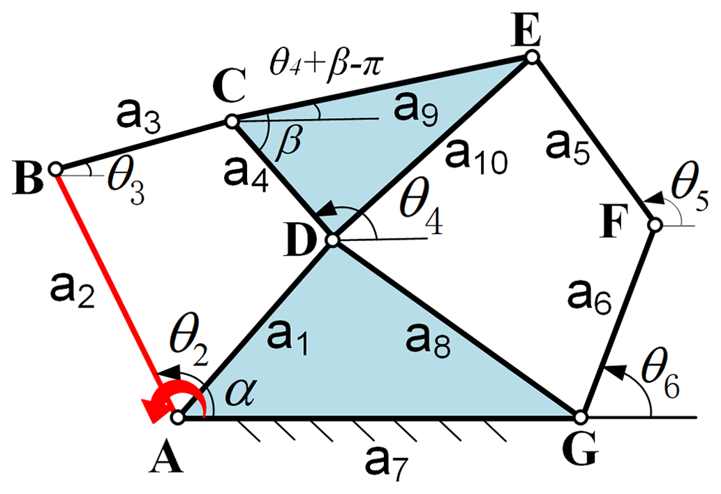
For the Stephenson six-bar planar mechanism in Fig. 8, the input joint is at joint A (i.e., the angle θ₂ is the input angle); two loop equations, which contain the all kinematic information of the mechanism, are shown as follows. The detailed calculation process for obtaining the one-to-one correspondence relationship equation between input and output joints or two input joints can be found in the published papers of our team (Ting and Dou, 1996; Ting et al., 2010; Wang et al., 2010).

For loop ABCD, we have

$$\begin{array}{}\text{(5)}& a_{\mathrm{2}}{e}^{i{\mathit{\theta }}_{\mathrm{2}}}+a_{\mathrm{3}}{e}^{i{\mathit{\theta }}_{\mathrm{3}}}-a_{\mathrm{1}}{e}^{i\mathit{\alpha }}-a_{\mathrm{4}}{e}^{i{\mathit{\theta }}_{\mathrm{4}}}=\mathrm{0},\end{array}$$

and for the loop ABEFG, we have,

$$\begin{array}{}\text{(6)}& a_{\mathrm{2}}{e}^{i{\mathit{\theta }}_{\mathrm{2}}}+a_{\mathrm{9}}{e}^{i\left(\mathit{\beta }+{\mathit{\theta }}_{\mathrm{5}}-\mathrm{2}\mathit{\pi }\right)}-a_{\mathrm{7}}-a_{\mathrm{6}}{e}^{i{\mathit{\theta }}_{\mathrm{6}}}-a_{\mathrm{5}}{e}^{i{\mathit{\theta }}_{\mathrm{5}}}=\mathrm{0}.\end{array}$$

2. Construction of Stephenson six-bar three-mode planar mechanism

According to the discussion in Sect. 3, constructing single-DOF MMPMs involves first identifying the bifurcation ability of the corresponding planar mechanism and then replacing the appropriate links or components with suitable MMMs to achieve mode conversion. For bifurcation ability, based on the loop equations above, the corresponding branch graph of the Stephenson six-bar planar mechanism can be obtained using Maple. Adjusting the link parameters of the Stephenson six-bar planar mechanism, a branch graph with three branches (branches I, II, and III) is shown in Fig. 9 (since the branch graph belongs to the 2π cycle of trigonometric functions, the two branch graphs can be shown as in Fig. 9 for the sake of intuitive analysis). In Fig. 9, the red curve is the joint rotation space of the four-bar loop ABCD, and the blue curve and inside part (light-gray area) are the joint rotation space of the five-bar loop DCEFG. The corresponding parameters of the Stephenson six-bar planar mechanism are listed in Table 4. For mode conversion, firstly, the singularity points are obtained by solving loop equations, that is, singularity points 1, 2, 3, 4, 5, 6, and 7 in Table 5. Furthermore, it is easy to see that the points 5^′, 6^′, and 7^′ are the same as the points 5, 6, and 7 in Fig. 9, and the three branches are separated by the singularity points 1, 2, 3, 4, 5, and 6 (branch points) listed in Table 5. In addiction, point 7 (Table 5) constitutes the sub-branch points that cannot affect the branches. Secondly, according to the singularity points and the input condition of the Stephenson six-bar planar mechanism, the continuities of the three branches are checked. Obviously, they are continuous. Then, the replaced links are chosen, that is, the links CD and EF, and the MMMs, i.e., the telescopic link-type module (II), are replaced as shown in Fig. 10. In Fig. 10, the structures of the telescopic link modules are not drawn in detail; i.e., they are represented as the purple links for the sake of simplification.

Figure 9 Branch graph of the Stephenson six-bar planar mechanism $(-\mathrm{2}\mathit{\pi }\le {\mathit{\theta }}_{\mathrm{2}}\le \mathrm{2}\mathit{\pi })$.

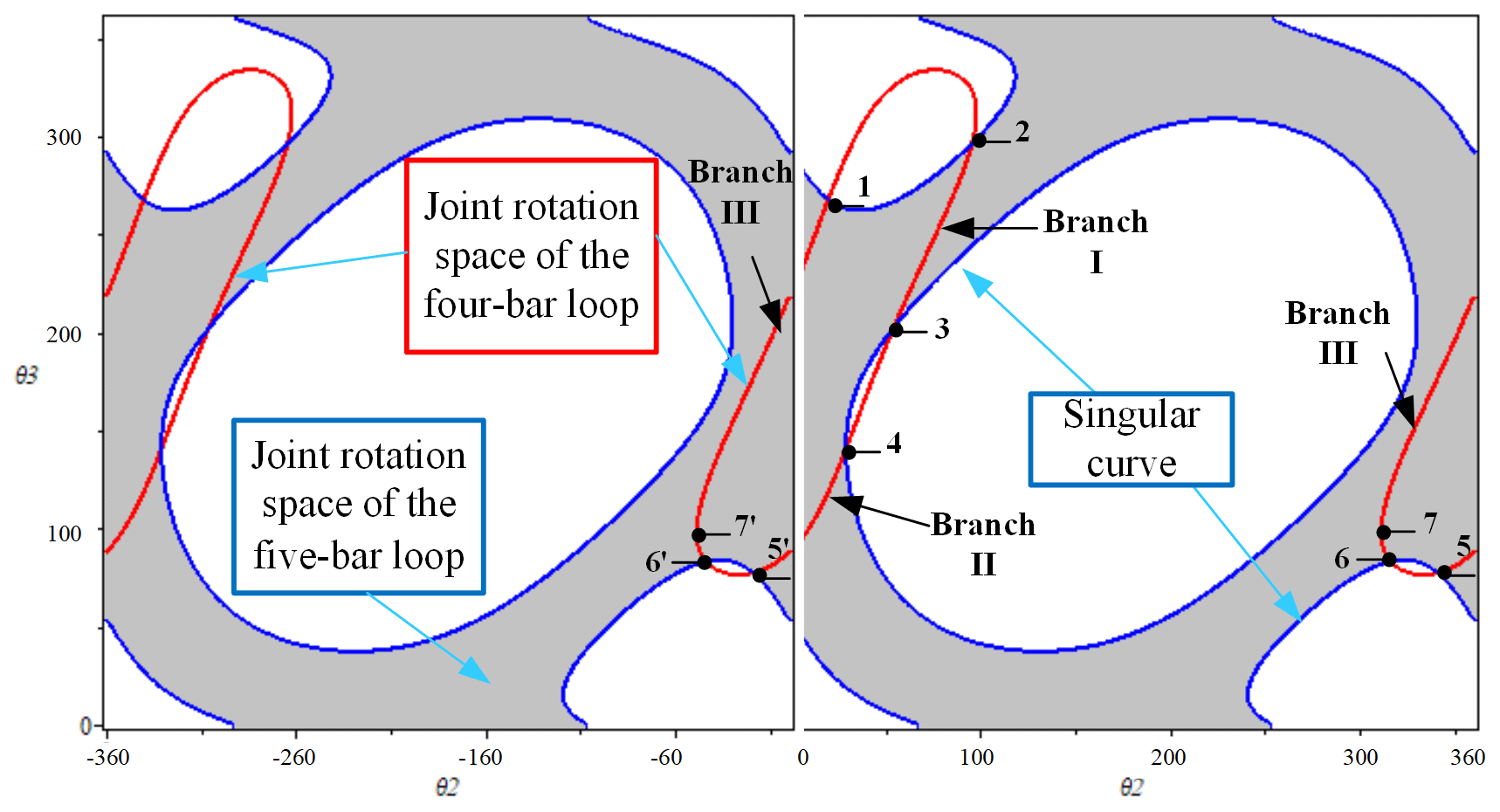
Table 4 Parameters of the Stephenson six-bar planar mechanism in Fig. 14.

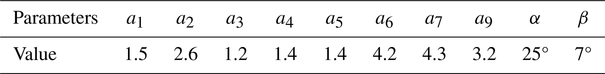
Table 5 Singularity points of the Stephenson six-bar planar mechanism.

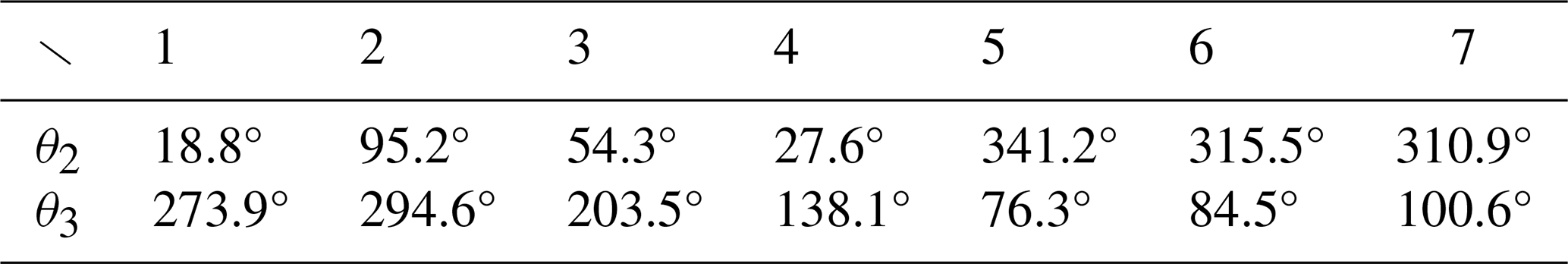
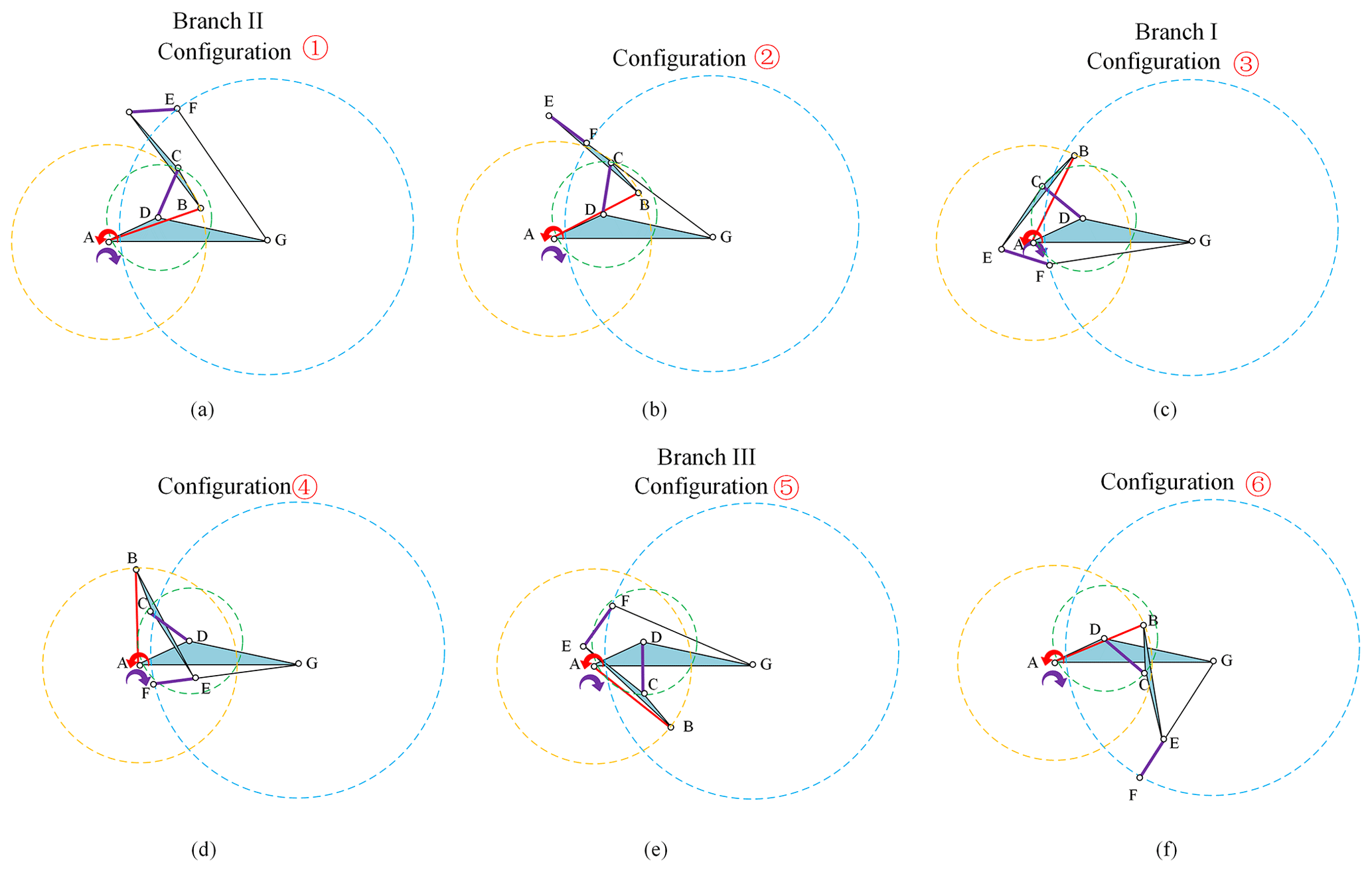
Figure 10 Several configurations of the Stephenson six-bar planar mechanism: (a) configuration ① (−18.8° $<{\mathit{\theta }}_{\mathrm{2}}<$ 27.6°), (b) configuration ② (θ₂= 27.6°), (c) configuration ③ (54.3° $<{\mathit{\theta }}_{\mathrm{2}}<$ 95.2°), (d) configuration ④ (θ₂=95.2°), (e) configuration ⑤ (310.9° $<{\mathit{\theta }}_{\mathrm{2}}<$ 18.8° +360°), and (f) configuration ⑥ (θ₂= 18.8° +360°).

3. Multi-mode motion analysis

The Stephenson six-bar MMPM (Fig. 10) has mainly six motion states: configurations ①, ②, ③, ④, ⑤, and ⑥ when the input link is link AB. Configuration ① represents the continuous-motion state within the input limit range of branch II (Fig. 10a), configuration ② represents the motion state at the singularity position of branch II (the passive links EF and FG come across in a straight line, i.e., the singularity point 4 in Fig. 10b), configuration ③ represents the continuous-motion state within the input limit of branch I (Fig. 10c), configuration ④ represents the motion state at the singularity position of branch I (the passive links EF and FG come across in a straight line, i.e., the singularity point 2 in Fig. 10d), configuration ⑤ represents the continuous-motion state within the input limit of branch III (Fig. 10e), and configuration ⑥ represents the motion state at the singularity position of branch III (the passive links EF and FG come across in a straight line, i.e., the singularity point 1 in Fig. 10f).

As the Stephenson six-bar MMPM only has three motion modes (branches), there are only six types of mode transitions, namely, (1) branch II → branch I, (2) branch I → branch III, (3) branch III → branch II, (4) branch I → branch II (5) branch III → branch I, and (6) branch II → branch III. Considering the above mode transitions, it is easy to find the fact that the first three can form the counterclockwise loop of mode conversion (i.e., branch II → branch I → branch III → branch II in Fig. 9; here, the symbol → shows the direction of motion state transformation), and the last three can establish the clockwise loop (branch II → branch III → branch I → branch II). If the input direction is given as a red arrow, indicating that the input is in full rotation, based on structural characteristics of the telescopic link module (I), the motion state loop configuration ① (branch II) → configuration ② → configuration ③ (branch I) → configuration ④ → configuration ⑤ (branch III) → configuration ⑥ → configuration ① can be formed. Since the only difference between the counterclockwise loop and the clockwise loop is the input direction, the following parts of the paper only discuss the counterclockwise loop case.

(1) Branch II to branch I. In the motion state configurations ① and ②, the telescopic link modules are in the original size state. The mechanism is in branch II (−18.8° (341.2–360°) $<{\mathit{\theta }}_{\mathrm{2}}<$ 27.6°). During the process of configuration ② transforming into configuration ③, firstly, the telescopic link module EF is in the variable-scale stretching state under the traction action reaching the longest length, and then it is compressed to the original size. Finally, the mechanism reaches configuration ③ (54.3° $<{\mathit{\theta }}_{\mathrm{2}}<$ 95.2°), that is, branch I.

(2) Branch I to branch III. In the process of configuration ④ transforming into Configuration ⑤, the telescopic link module EF undergoes the process of stretching to the bottom and then compressing to the original size. Then the mechanism moves into branch III.

(3) Branch III to branch II. In the process of configuration ⑤ transforming into configuration ①, as the input link continues to rotate, the mechanism will meet configuration ⑥, and then the telescopic link module EF is stretched to break the singularity position (the configuration of singularity point 5), leading to the MMPM transforming from branch III to branch II. Particularly worth mentioning is that the singularity point 7 in branch III is the sub-branch point; that is, there are two sub-branches (sub-branch 1-7 and sub-branch 7-6). As is known from the discussion in Sect. 2.2, they can appear at the same time. Therefore, in this case, the sub-branch 1-7 is chosen, which mean the singularity point 1 (configuration ⑥) will be met in the in the process of configuration ⑤ transforming into configuration ①.

According to the discussion above, considering the input direction given (red arrow), as shown in Fig. 10, the Stephenson six-bar MMPM only meets the singularity points 4, 2, and 1 or 6 in order (forming the branch II → branch I → branch III → branch II loop), and only the telescopic link module EF works, but the singularity points 3, 5, and 7 are missing. The reason is that the configuration of the mechanism is different under conditions of different input direction (see the discussion of the four-bar case in Fig. 7a). In other words, the Stephenson six-bar MMPM will only meet the singularity points 3, 5, and 7 and will lose the points 4, 2, and 1 or 6 if the input direction is reversed (purple arrow) in Fig. 10 (forming the branch II → branch III → branch I → branch II loop), and at the singularity point 7, the telescopic link module CD will be used to break the constraint singularity of the mechanism.

In short, using the proposed method for the Stephenson six-bar MMPM, the mechanism will transform from branch I to branch II when the mechanism breaks through the singularity point 4 (Fig. 10b). When the mechanism breaks through the singularity point 2 (Fig. 10d), the mechanism will switch from branch I to branch III.

4.1.2 Single-degree-of-freedom Watt six-bar three-mode planar mechanism

1. Loop equation established

For the Watt six-bar planar mechanism in Fig. 11, the input joint is at the joint A (i.e., the angle θ₂ is the input angle); two loop equations, which contain the all kinematic information of the mechanism, are shown as follows. For the detailed calculation process, the reader can refer to the published papers of our team (Wang et al., 2014).

Figure 11 Kinematic graph of the Watt six-bar planar mechanism.

For the loop ABCD, we have

$$\begin{array}{}\text{(7)}& a_{\mathrm{2}}{e}^{i{\mathit{\theta }}_{\mathrm{2}}}+a_{\mathrm{3}}{e}^{i{\mathit{\theta }}_{\mathrm{3}}}-a_{\mathrm{1}}{e}^{i\mathit{\alpha }}-a_{\mathrm{4}}{e}^{i{\mathit{\theta }}_{\mathrm{4}}}=\mathrm{0},\end{array}$$

and for the loop ABEFG, we have

$$\begin{array}{}\text{(8)}& a_{\mathrm{2}}{e}^{i{\mathit{\theta }}_{\mathrm{2}}}+a_{\mathrm{3}}{e}^{i{\mathit{\theta }}_{\mathrm{3}}}+a_{\mathrm{9}}{e}^{i\left({\mathit{\theta }}_{\mathrm{4}}+\mathit{\beta }-\mathit{\pi }\right)}-a_{\mathrm{7}}-a_{\mathrm{5}}{e}^{i{\mathit{\theta }}_{\mathrm{5}}}-a_{\mathrm{6}}{e}^{i{\mathit{\theta }}_{\mathrm{6}}}=\mathrm{0}.\end{array}$$

2. Construction of Watt six-bar three-mode planar mechanism

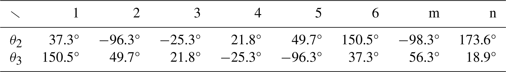
Similarly to the Stephenson six-bar planar mechanism case, to construct the Watt six-bar three-mode planar mechanism, the two conditions regarding bifurcation motion and mode conversion also need to be satisfied. (1) For bifurcation motion, by adjusting the link parameters of the Watt six-bar planar mechanism, a branch graph with three branches (branches I, II, and III) is shown in Fig. 12. In Fig. 12, the red curve is the joint rotation space of the four-bar loop ABCD, and the blue curve and inside part (light-gray area) are the joint rotation space of the virtual five-bar loop ABEFG. The corresponding parameters of the Watt six-bar planar mechanism are listed in Table 6. For mode conversion, the singularity points are obtained solving loop Eqs. (7) and (8), that is, singularity points 1, 2, 3, 4, 5, 6, m, and n in Table 7. Additionally, the three branches are separated by the singularity points 1, 2, 3, 4, 5, and 6. These points are the branch points. Furthermore, points m and n are the sub-branch points. In addiction, the replaced links are the links BC and EF, and the corresponding Watt six-bar three-mode planar mechanisms are obtained and shown in Fig. 13 with the MMMs, i.e., telescopic link-type module (II).

Figure 12 Branch graph of the Watt six-bar planar mechanism $(-\mathit{\pi }\le {\mathit{\theta }}_{\mathrm{2}}\le \mathit{\pi })$.

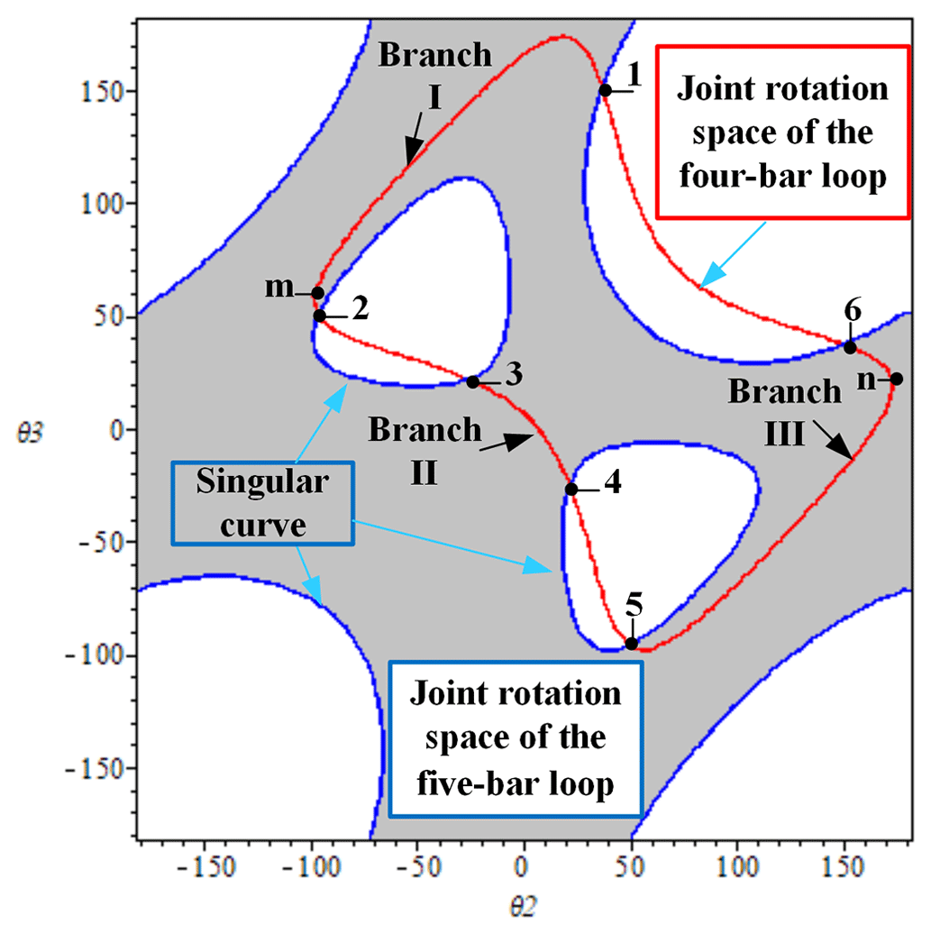
Table 6 Parameters of the Watt six-bar planar mechanism in Fig. 12.

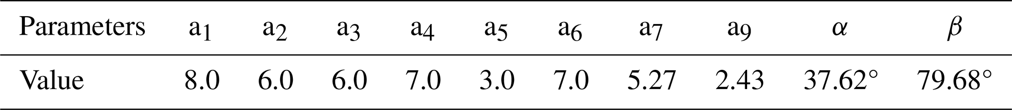
Table 7 Singularity points of the Watt six-bar planar mechanism.

3. Multi-mode motion analysis

The Watt six-bar MMPM (Fig. 13) has mainly six motion states: configurations ①, ②, ③, ④, ⑤, and ⑥ when the input link is link AB. Configuration ① represents the continuous-motion state within the input limit range of branch II (Fig. 13a), configuration ② (Fig. 13b) represents the motion state at the singularity position of branch II (the passive links EF and FG come across in a straight line, i.e., the singularity point 4 in Fig. 12), configuration ③ represents the continuous-motion state within the input limit of branch I (Fig. 13c), configuration ④ (Fig. 13d) represents the motion state at the singularity position of branch I (the passive links BC and CD come across in a straight line, i.e., the singularity point n in Fig. 12), configuration ⑤ represents the continuous-motion state within the input limit of branch III (Fig. 13e), configuration ⑥ (Fig. 13f) represents the motion state at the singularity position of branch III (the passive links EF and FG come cross in a straight line, i.e., the singularity point 2 in Fig. 12).

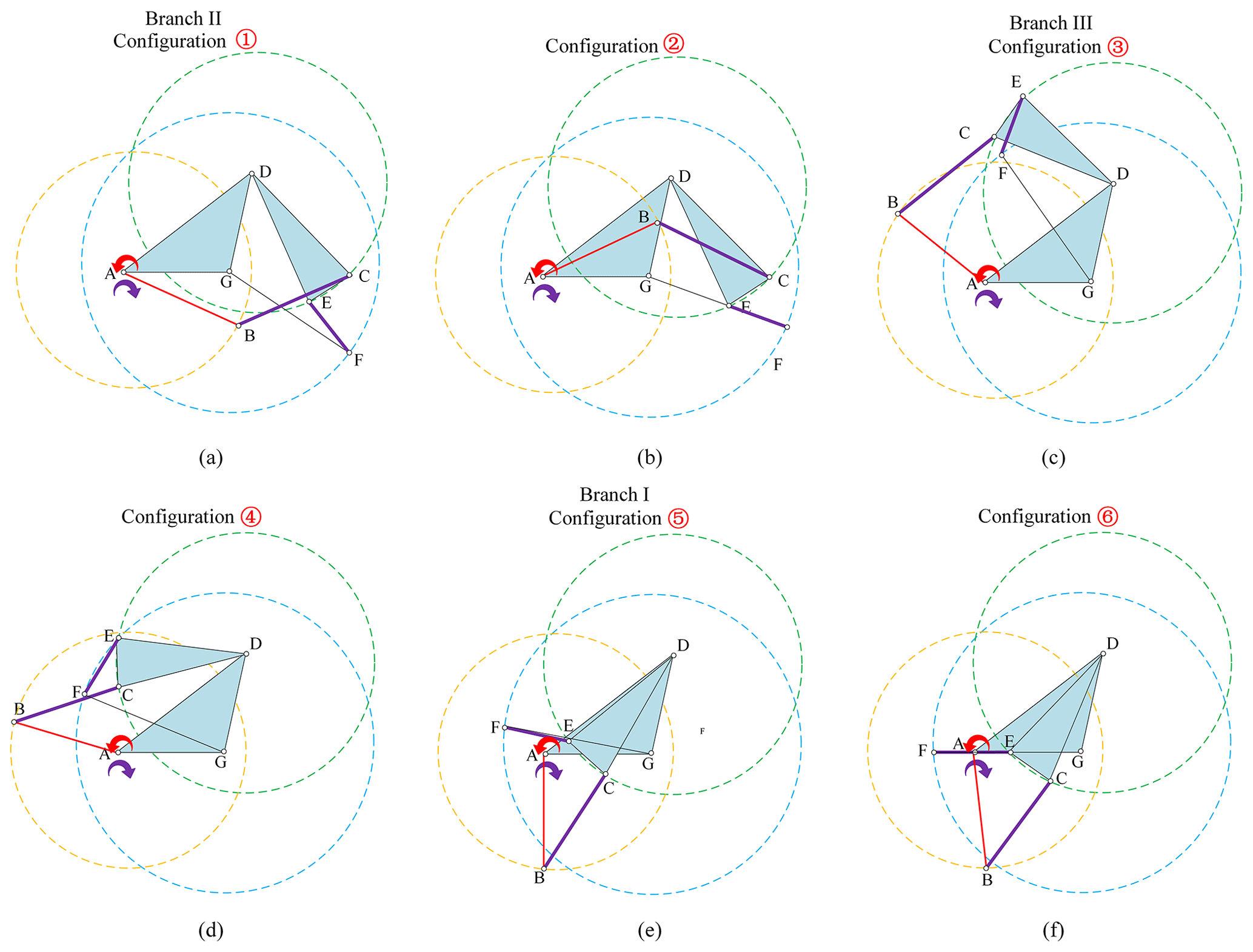
Figure 13 Several configurations of the Watt six-bar planar mechanism: (a) configuration ① (−25.3° $<{\mathit{\theta }}_{\mathrm{2}}<$ 21.8°), (b) configuration ② (θ₂= 21.8°), (c) configuration ③ (49.7° $<{\mathit{\theta }}_{\mathrm{2}}<$ 173.6°), (d) configuration ④ (θ₂= 173.6°), (e) configuration ⑤ (−98.3° + 360° $<{\mathit{\theta }}_{\mathrm{2}}<$ −96.3° + 360°), and (f) configuration ⑥ (θ₂= −96.3° + 360°).

Similarly to the Stephenson six-bar MMPM discussed above, the Watt six-bar MMPM also has three motion modes (branches); there are only six types of mode transitions, namely, (1) branch II to branch I, (2) branch I to branch III, (3) branch III to branch II, (4) branch I to branch II (5) branch III to branch I, and (6) branch II to branch III. Due to the same reason as the above case, here we only discuss the counterclockwise loop of the mode conversion case (i.e., branch II → branch III → branch I → branch II in Fig. 12); the corresponding motion state loop is configuration ① (branch II) → configuration ② → configuration ③ (branch I) → configuration ④ → configuration ⑤ (branch III) → configuration ⑥ → configuration ① loop.

(1) Branch II to branch III. In the motion state configurations ① and ②, the telescopic link modules are in the original size state. The mechanism is in branch II (−25.3° $<{\mathit{\theta }}_{\mathrm{2}}<$ 21.8°). During the process of configuration ② transforming into configuration ③, firstly, the telescopic link modules EF and BC are in the variable-scale stretching state under the traction action reaching the longest length, and then they are compressed to the original size (what is worth noting is that, in the process of mode conversion, the dimension change is generally completed by a single MMM, but in the above case, two MMMs are involved; the reason for this is that the passive links BC and CD also appear collinearly during the rotation of the mechanism, which leads to the emergence of new singularity). Finally, the mechanism reaches configuration ③ (49.7° $<{\mathit{\theta }}_{\mathrm{2}}<$ 173.6°), that is, branch III.

(2) Branch III to branch I. In the process of configuration ④ transforming into configuration ⑤, the telescopic link module BC undergoes the process of stretching to the bottom and then compressing to the original size. Then the mechanism moves into branch I.

(3) Branch I to branch II. In the process of configuration ⑤ transforming into configuration ①, as the input link continues to rotate, the mechanism will meet configuration ⑥, and then the telescopic link module EF is stretched to break the constraint singularity configuration (i.e., the configuration of singularity point 2), leading to the MMPM transforming from branch I into branch II.

According to the discussion above, considering the input direction given (red arrow), as shown in Fig. 13, the Watt six-bar MMPM only meets the singularity points 4, n, and 2 in order (forming the branch II → branch III → branch I → branch II loop), and the singularity points 3, m, and 6 are missing. The reason is that the configuration of the mechanism is different under conditions of different input directions. In other words, the Watt six-bar MMPM will only meet the singularity points 3, m, and 6 and will lose the points 4, n, and 2 if the input direction is reversed (purple arrow), as shown in Fig. 13. Note that 1-m and m-2 are the two sub-branches of branch I, which cannot exist at the same time; for that reason, the singularity points 1 and 2 can only appear once, and this paper takes singularity point 2 as an example. The same thing happened in the singularity points 5 and 6.

4.2 Single-degree-of-freedom eight-bar four-mode planar mechanisms

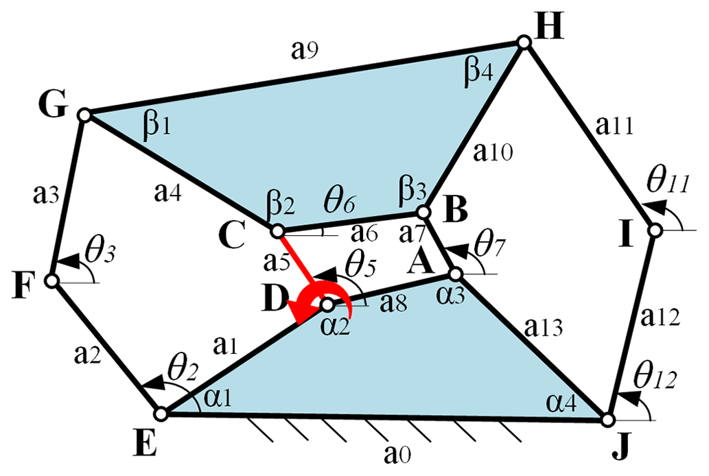
Single-DOF eight-bar planar mechanisms have 16 types of mechanism configurations based on Pennock and Hasan (2002). They usually consist of three loops. These loops may be composed of four bars, five bars, or even more bars. However, in this paper, because the branch graph of the mechanism is obtained by solving the corresponding input–output loop equations, only some single-DOF eight-bar planar mechanisms containing at least a four-bar loop and five-bar loops are suitable for this method. For that reason, the single-DOF eight-bar planar mechanism in Fig. 14, which consists of a four-bar loop and two five-bar loops, is taken as an example to explain the construction of single-DOF eight-bar MMPM.

Figure 14 Kinematic graph of an eight-bar planar mechanism.

1. Loop equation established

For the eight-bar planar mechanism in Fig. 14, the input joint is at the joint D (i.e., the angle θ₅ is the input angle); three loop equations, which contain the all kinematic information of the mechanism, are shown as follows. For the detailed calculation process, the reader can refer to the published papers of our team (Wang and Ting, 2002).

For loop DCBA, we have

$$\begin{array}{}\text{(9)}& a_{\mathrm{5}}{e}^{i{\mathit{\theta }}_{\mathrm{5}}}+a_{\mathrm{6}}{e}^{i{\mathit{\theta }}_{\mathrm{6}}}-a_{\mathrm{8}}{e}^{i\left({\mathit{\alpha }}_{\mathrm{1}}+{\mathit{\alpha }}_{\mathrm{2}}-\mathit{\pi }\right)}-a_{\mathrm{7}}{e}^{i{\mathit{\theta }}_{\mathrm{7}}}=\mathrm{0}.\end{array}$$

For loop EFGCD, we have

$$\begin{array}{}\text{(10)}& a_{\mathrm{2}}{e}^{i{\mathit{\theta }}_{\mathrm{2}}}+a_{\mathrm{3}}{e}^{i{\mathit{\theta }}_{\mathrm{3}}}+a_{\mathrm{4}}{e}^{i\left(\mathit{\pi }+{\mathit{\beta }}_{\mathrm{2}}+{\mathit{\theta }}_{\mathrm{6}}\right)}-a_{\mathrm{1}}{e}^{i{\mathit{\alpha }}_{\mathrm{1}}}-a_{\mathrm{5}}{e}^{i{\mathit{\theta }}_{\mathrm{5}}}=\mathrm{0}.\end{array}$$

For loop DCBHIJAD, we have

$$\begin{array}{}\text{(11)}& \begin{array}{rl}& a_{\mathrm{5}}{e}^{i{\mathit{\theta }}_{\mathrm{5}}}+a_{\mathrm{6}}{e}^{i{\mathit{\theta }}_{\mathrm{6}}}+a_{\mathrm{10}}{e}^{i\left(\mathit{\pi }-{\mathit{\beta }}_{\mathrm{3}}+{\mathit{\theta }}_{\mathrm{6}}\right)}-a_{\mathrm{8}}{e}^{i\left(\mathit{\pi }-{\mathit{\alpha }}_{\mathrm{3}}-{\mathit{\alpha }}_{\mathrm{4}}\right)}\\ & -a_{\mathrm{13}}{e}^{i\left(\mathrm{2}\mathit{\pi }-{\mathit{\alpha }}_{\mathrm{4}}\right)}-a_{\mathrm{12}}{e}^{i{\mathit{\theta }}_{\mathrm{12}}}-a_{\mathrm{11}}{e}^{i{\mathit{\theta }}_{\mathrm{11}}}=\mathrm{0}.\end{array}\end{array}$$

2. Construction of eight-bar four-mode planar mechanism

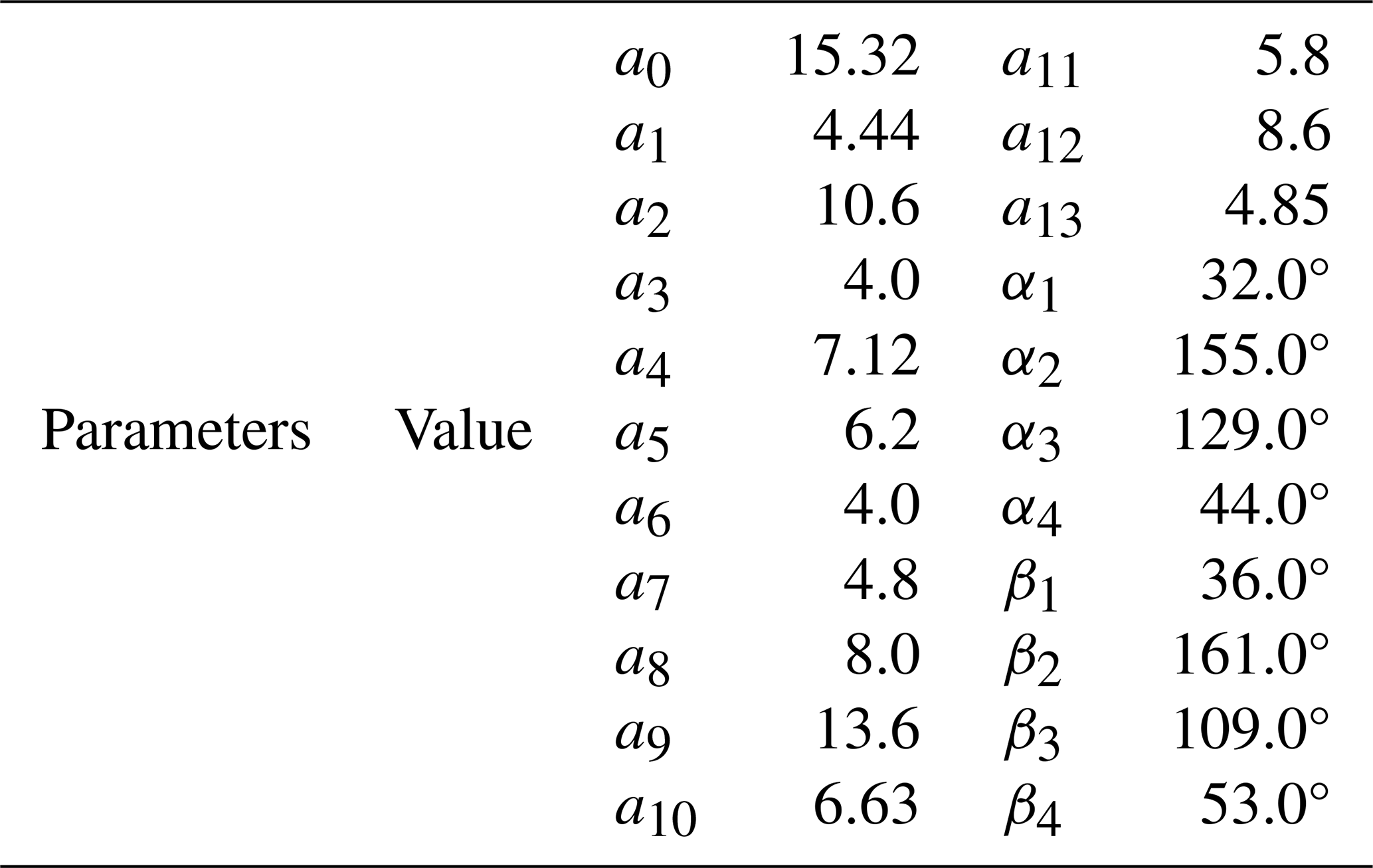
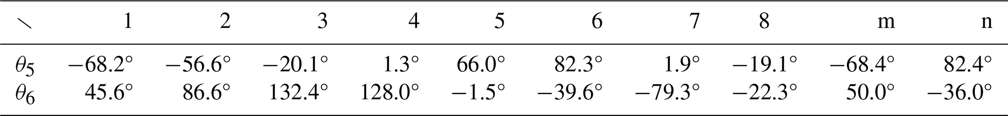
Firstly, to satisfy the requirement of bifurcation motion, for the eight-bar planar mechanism in Fig. 14, the branch graph with four branches (branches I, II, III, and IV) is shown in Fig. 15. In Fig. 15, the red curve is the joint rotation space (JRS) of the four-bar loop DCBA; the blue curve and inside part (light-blue area) are the JRS of the five-bar loop EFGCD; the green curve and inside part (light-green area) are the JRS of the seven-bar loop DCBHIJAD (it is actually a virtual five-bar loop); and the common part of the three JRSs is the actual JRS where the mechanism can move, that is, the four branches: branch I, II, III, and IV. The corresponding parameters of the eight-bar planar mechanism are listed in Table 8. Secondly, for the requirement of mode conversion, the singularity points are obtained by solving loop Eqs. (9), (10), and (11), that is, singularity points 1, 2, 3, 4, 5, 6, 7, 8, m, and n in Table 9. The singularity points 1, 2, 3, 4, 5, 6, 7, and 8 are the branch points, which separate the four branches. Points m and n are the sub-branch points. In addiction, the replaced links are the links FG, BA, and HI, and the corresponding eight-bar four-mode planar mechanisms are obtained and shown in Fig. 16 with the MMMs, i.e., telescopic link-type module (II).

Figure 15 Branch graph of the eight-bar planar mechanism.

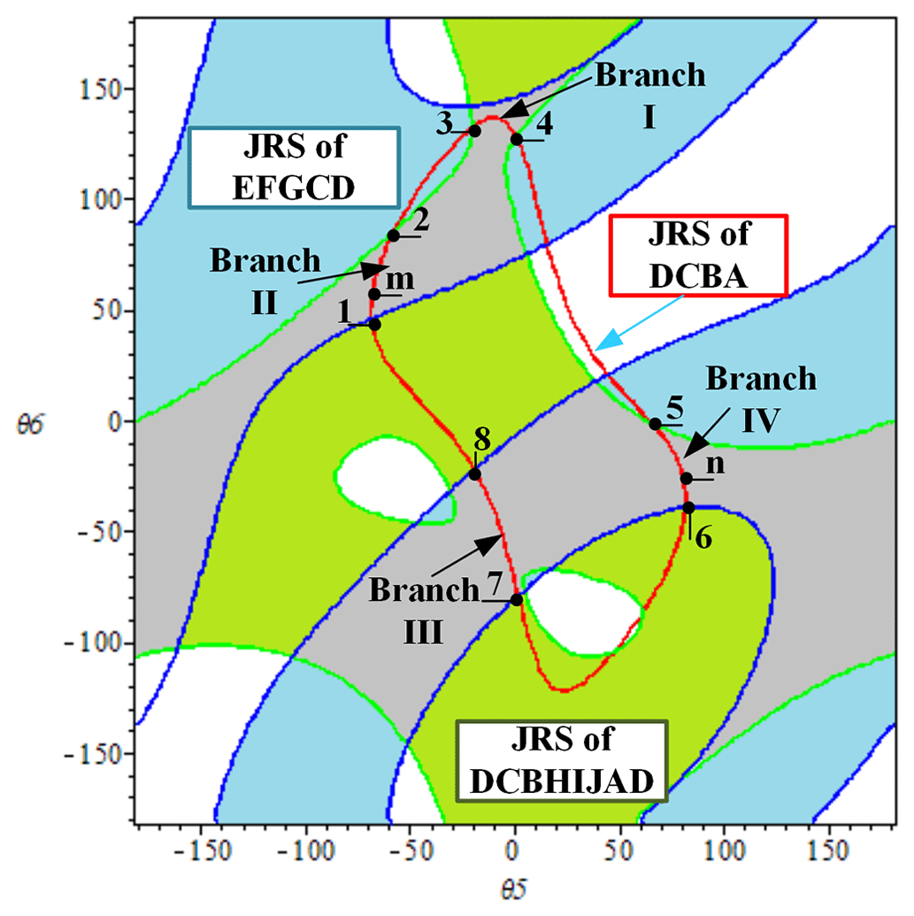
Table 8 Parameters of the eight-bar planar mechanism in Fig. 15.​​​​​​​

Table 9 Singularity points of the eight-bar planar mechanism.

3. Multi-mode motion analysis

The eight-bar MMPM (Fig. 16) has mainly eight motion states: configurations ①, ②, ③, ④, ⑤, ⑥, ⑦, and ⑧ when the input link is link DC (i.e., the red link). Configuration ① represents the continuous-motion state within the input limit range of branch I (Fig. 16a), configuration ② (Fig. 16b) represents the motion state at the singularity position of branch I (the passive links HI and IJ come across in a straight line, i.e., the singularity point 4 in Fig. 15), configuration ③ represents the continuous-motion state within the input limit of branch IV (Fig. 16c), configuration ④ (Fig. 16d) represents the motion state at the singularity position of branch IV (the passive links BC and AB come across in a straight line, i.e., the singularity point n in Fig. 15), configuration ⑤ represents the continuous-motion state within the input limit of branch II (Fig. 16e), and configuration ⑥ (Fig. 16f) represents the motion state at the singularity position of branch II (the passive links HI and IJ come across in a straight line, i.e., the singularity point 2 in Fig. 15).

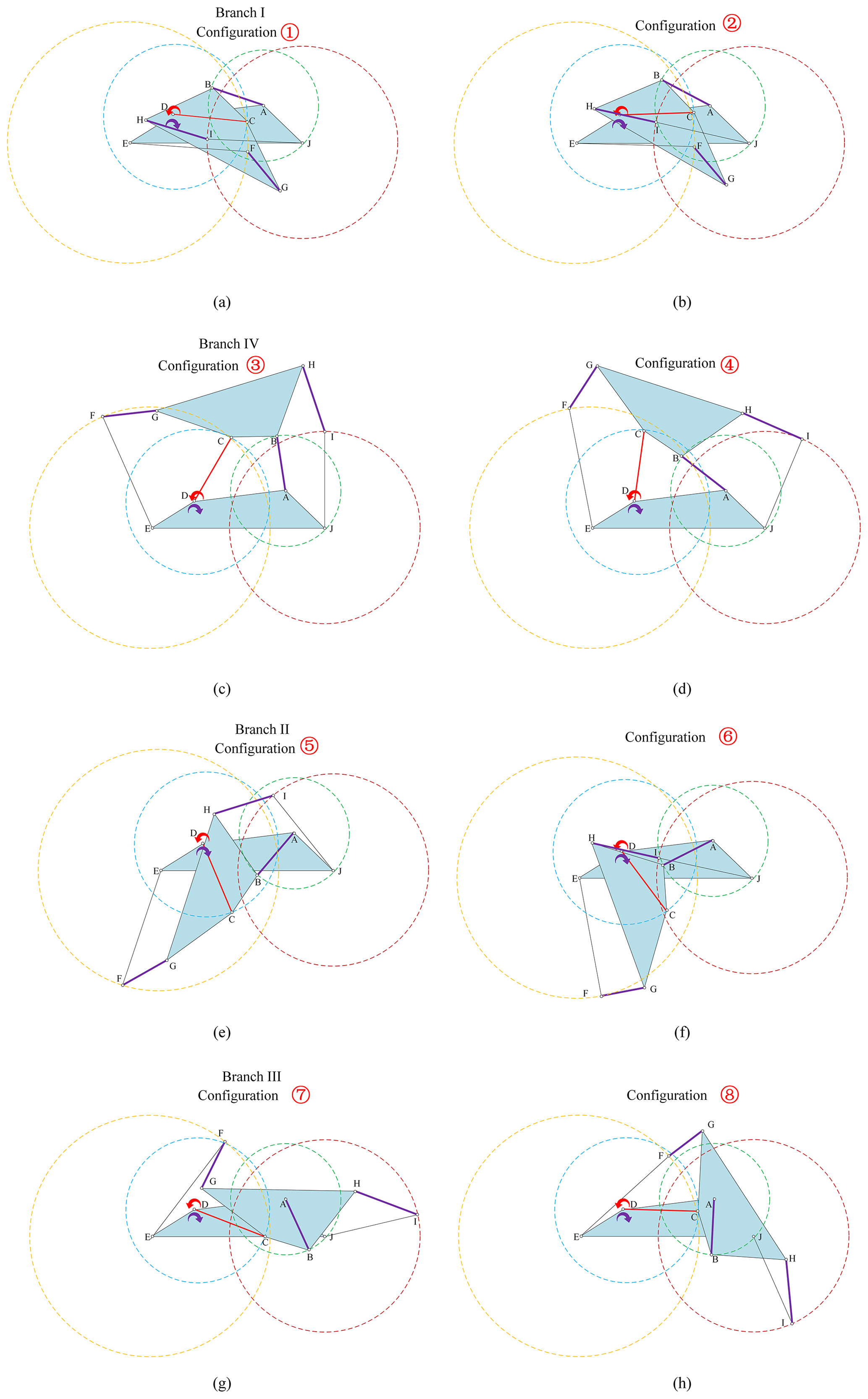
Figure 16 Several configurations of the eight-bar planar mechanism: (a) configuration ① (−20.1° $<{\mathit{\theta }}_{\mathrm{5}}<$ 1.3°), (b) configuration ② (θ₅= 1.3°), (c) configuration ③ (66.0° $<{\mathit{\theta }}_{\mathrm{5}}<$ 82.4°), (d) configuration ④ (θ₅= 82.4°), (e) configuration ⑤ (−68.4° + 360° $<{\mathit{\theta }}_{\mathrm{5}}<$ −56.6° + 360°), (f) configuration ⑥ (θ₅= −56.6° + 360°), (g) configuration ⑦ (−19.1° + 360° $<{\mathit{\theta }}_{\mathrm{5}}<$ 1.9° + 360°), and (h) configuration ⑧ (θ₅= 1.9° + 360°).

According above stated, the eight-bar MMPM has four motion modes (branches); in general, there are only eight types of mode transitions, namely, (1) branch I to branch IV, (2) branch IV to branch II, (3) branch II to branch III, (4) branch III to branch I, (5) branch I to branch III, (6) branch III to branch II, (7) branch II to branch IV, and (8) branch IV to branch I. However, in this case, since this MMPM has the common part of the input angle range between branch I (−20.1° $<{\mathit{\theta }}_{\mathrm{5}}<$ 1.3°) and branch III (−19.1° $<{\mathit{\theta }}_{\mathrm{5}}<$ 1.9°), in a cycle (2π), the transformation from branch III into branch I cannot proceed directly; that is, counterclockwise loop (formed by (1), (2), (3), and (4)) of branch I → branch IV → branch II → branch III → branch I cannot be formed. Instead, the following loop of branch I → branch IV → branch II → branch III → branch IV → branch II → branch III is formed. Furthermore, for the same reason, the probability of the MMPM switching from branch IV to branch I and branch III is random when the MMPM is in a clockwise loop (i.e, branch I → branch III → branch II → branch IV → branch I). That is a very interesting question, but because it is not the focus of this article, the discussion is not expanded. Here, we only discuss the simple motion state loop of configuration ① → configuration ② → configuration ③ → configuration ④ → configuration ⑤ → configuration ⑥ → configuration ⑥ → configuration ⑦ → configuration ⑧ → configuration ③, that is, branch I → branch IV → branch II → branch III → branch IV → branch II → branch III.

(1) Branch I to branch IV. In the motion state configurations ① and ② , the telescopic link modules are in the original size state. The mechanism is in branch I (−20.1° $<{\mathit{\theta }}_{\mathrm{5}}<$ 1.3°). During the process of configuration ② transforming into configuration ③, firstly, the telescopic link module HI is in the variable-scale stretching state under the traction action reaching the longest length, and then it is compressed to the original size. Finally, the mechanism reaches configuration ③ (66.0° $<{\mathit{\theta }}_{\mathrm{2}}<$ 82.4°), that is, branch IV.

(2) Branch IV to branch II. In the process of configuration ④ transforming into configuration ⑤, the telescopic link module AB undergoes the process of stretching to the bottom and then compressing to the original size. Then the mechanism moves into branch III.

(3) Branch II to branch III. In the process of configuration ⑤ transforming into configuration ⑦, as the input link continues to rotate, the mechanism will meet configuration ⑥, and then the telescopic link module HI is stretched to break the constraint singularity configuration (i.e., the configuration of singularity point 2), leading to the MMPM transforming from branch II to branch III.

(4) Branch III to branch IV. In the process of configuration ⑦ transforming into configuration ③, the mechanism will meet configuration ⑧, and then the telescopic link module FG is stretched to break the constraint singularity configuration (i.e., the configuration of singularity point 7), leading to the MMPM transforming from branch III into branch IV.

The remaining mode transitions of branch IV to branch II and branch II to branch III in the above-mentioned simple motion state loop are the same as in the cases of (2) branch IV to branch II and (3) branch II to branch III.

According to the discussion above, considering the input direction given (red arrow), as shown in Fig. 16, the eight-bar MMPM only meets the singularity points 4 and n or 5, 2, and 7 in order (forming the branch I → branch IV → branch II → branch III → branch IV → branch II → branch III loop), and the singularity points 8 and m or 1, 3, and 6 are missing. The reason is that the configuration of the mechanism is different under conditions of different input directions. In other words, the eight-bar MMPM will only meet the singularity points 8, m, 3, and 6 and will lose the points 4, n, 2, and 7 if the input direction is reversed (purple arrow), as shown in Fig. 16. Normally, since the singularity points m and n are sub-branch points, the singularity points 1 and 2 can appear at the same time. The singularity points 5 and 6 experienced the same occurrence. However, in this case, except for the above situation, the singularity points 1 and m and 5 and n, which are the two extreme points of the same sub-branches, also cannot exist at the same time in a mode transition. The reason for this is that the corresponding angles θ₅ of the two are too close, causing the mechanism to be bound to miss one of them in the mode conversion. As a result, the singularity points 1 and m can only appear once, and this paper takes singularity point m as an example. The same thing happened in the singularity points 5 and n.

5 Conclusions

Based on loop equations and branch graphs, this paper proposes a method to construct some single-DOF MMPMs by replacing links or components of the singular configuration of corresponding planar mechanisms with the MMMs. The conclusions and advantages can be summarized as follows.

• 1.

  Due to the corresponding bifurcation analysis and mode conversion of this method only depending on the branch graphs, singularity points, and the replacing MMMs (all three are common to planar mechanisms), the proposed method is straightforward and visible and can be widely applicable to single-DOF MMPM.

• 2.

  For the potential bifurcation and mode conversion ability of planar mechanisms, this paper provides the specific identification index (i.e., the number and continuity of branches), which will give a new design direction and powerful design guidance for the design of MMPMs.

• 3.

  A single-DOF four-bar MMPM, a single-DOF Stephenson six-bar three-mode planar mechanism, a Watt six-bar three-mode planar mechanism, and an eight-bar four-mode planar mechanism are constructed. The last three MMPMs are formed for the first time. The results provide more choices for the available configuration and its application.