Development of a flexible endoscopic robot with autonomous tracking control ability using machine vision and deep learning

A flexible endoscopic robot is designed to solve the problem that it is difficult for auxiliary doctors to maintain a stable visual field in traditional endoscopic surgery. Based on geometric derivation, a motion control method under the constraint of the remote center motion (RCM) of the robot system is established, and a set of circular trajectories are planned for it. The RCM error of the robot during operation and the actual trajectory of the robot end in three-dimensional space are obtained through the motion capture system. The end of the robot is controlled by the heterogeneous primary–secondary teleoperation control algorithm based on position increments. Finally, the RTMDet deep learning object detection algorithm was selected to identify and locate surgical instruments through comparative experiments, and the autonomous tracking control was completed based on visual guidance. In the process of autonomous tracking, the RCM error was less than 1 mm, which met the actual surgical requirements.

1 Introduction

Compared with traditional open surgery, endoscopic minimally invasive surgical robots (EMISRs) have many advantages, such as less surgical trauma, less blood loss and faster recovery (Ejaz et al., 2014; Zenoni et al., 2013). The research of endoscopic minimally invasive surgical robots not only has high academic value but also has a broad market prospect and great economic benefits (Dhumane et al., 2011; Gomes, 2011). Many well-known universities, enterprises and other institutions have started to conduct in-depth research on endoscopic surgical robots, which involves various aspects such as mechanical design, kinematic modeling, drive compensation, motion control, force sensing and automatic tracking.

With the improvements in accuracy and reliability, endoscopic surgical robotic systems have achieved more significant research results, and the related achievements have been put into use in hospitals, providing great help to doctors. For example, based on the AESOP surgical system, the Computer Motion company developed the ZEUS surgical system and performed the famous removal procedure “Lindbergh operation” (Guthart and Salisbury, 2000; Sung and Gill, 2001). The da Vinci surgical system was successfully developed by Intuitive Surgical in the United States, which has been approved by the FDA for use in hospitals (Brahmbhatt et al., 2014; Chen et al., 2018; Freschi et al., 2013). Tianjin University and Tianjin Medical University jointly developed the surgical robot “MicroHand S” system (Li et al., 2005; Liang et al., 2018; Su et al., 2018), which adopts a primary–secondary heterogeneous spatial mapping model and has virtual force feedback function.

Compared with traditional rigid joints, the flexible continuum mechanism has the advantages of light weight, high integration and high flexibility of motion. Olympus Medical, Japan, developed a flexible endoscope whose bending motion is controlled by a set of wires (Zhang et al., 2011). Based on this, several flexible instruments and endoscopes have been developed by related organizations in Berkelman and Ma (2009), Ding et al. (2012), Dai et al. (2019), Wang et al. (2023) and Kanno et al. (2014). A flexible laparoscopic robot was proposed which can capture images flexibly in Tewari et al. (2013).

Flexible endoscopic robots are constrained by the remote center of motion (RCM) during motion. Dedicated medical surgical robots generally use special mechanical structures (e.g., parallelogram mechanism or spherical mechanism) to achieve the RCM constraint (Tewari et al., 2013). Since medical surgical robots are expensive, in this paper, we want to use a general-purpose robotic arm instead of a dedicated surgical robot and implement the RCM constraint using a programmable algorithm (Sandoval et al., 2016; Sadeghian et al., 2019; Aghakhani et al., 2013).

The main contribution of this research is to realize the motion planning and primary–secondary teleoperation control of the flexible endoscope robot under RCM constraints on the basis of the structure of the flexible endoscope robot and select the appropriate deep learning algorithm to complete the autonomous tracking function. Firstly, the inverse kinematics solution of the robot arm under the constraint of RCM is derived, and the trajectory planning of the flexible endoscope robot is verified. In addition, considering the preoperative position and teleoperation control strategy, a primary–secondary teleoperation control system constrained by RCM was established. At the same time, machine vision and deep learning technology were applied to the flexible endoscope robot, and the autonomous tracking control strategy based on vision guidance is proposed and verified. The details are as follows: Sect. 1 is an introduction, Sect. 2 details the flexible endoscopic robot design, Sect. 3 details a flexible endoscopic robot motion planning and teleoperation experiment, Sect. 4 details a flexible endoscopic robot autonomous tracking control experiment, and Sect. 5 concludes the paper.

2 Flexible endoscopic robot design

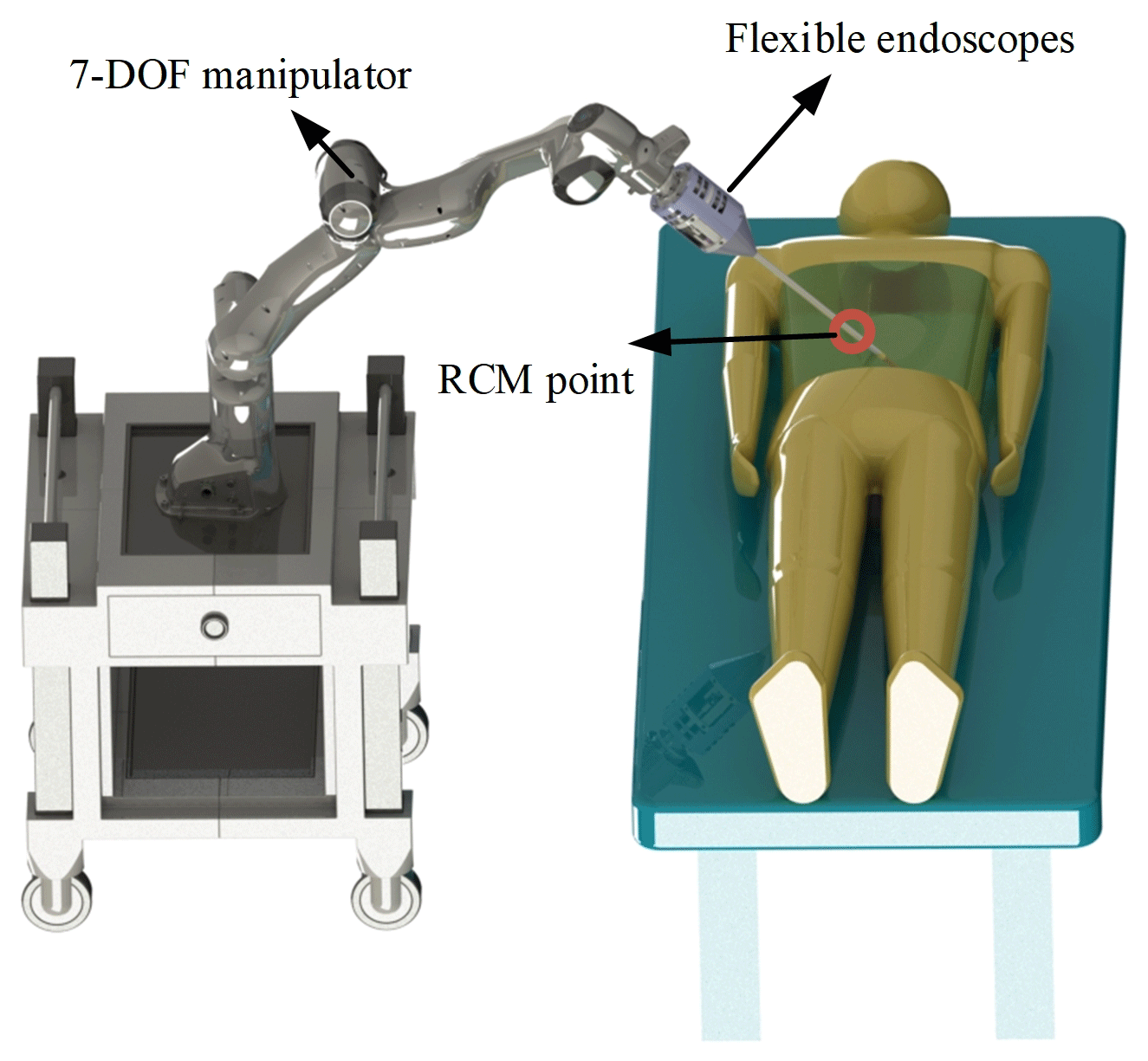
In traditional minimally invasive endoscopic surgery, the movement flexibility of the endoscope is limited by the telecentric point, and it is difficult to flexibly adjust the specific position of the end lens in the abdominal cavity. Therefore, in order to enhance the movement flexibility of the endoscope and the stability of the visual field and meet the requirements of doctors for the surgical visual field, the structural design of Shiyang Bao (2023) is quoted in this paper, and the RCM constraint is realized using a universal robotic arm. The overall structure is shown in Fig. 1.

Figure 1 Schematic diagram of the overall flexible endoscopic robot.

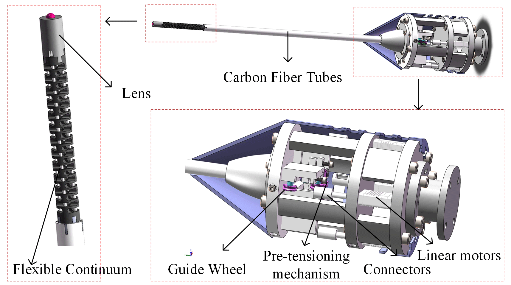
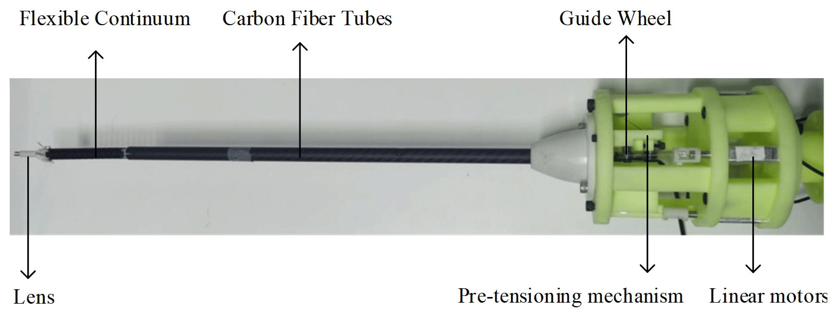
The overall structure of the 2 degrees of freedom (DOF) flexible endoscope actuator is shown in Fig. 2, which specifically includes a flexible continuum, a lens, a carbon fiber tube, a preload mechanism, a guide wheel, a micro linear motor and a fixing device. Four micro linear motors are evenly arranged, with one section of the flexible cable connected to the micro linear motor and the other end passing through the guide wheel and the carbon fiber tube and finally passing through the flexible continuum fixed with a threaded aluminum sleeve. The preload mechanism consists of preload slider and preload screw. By rotating the preload screw, it drives the preload slider to move, which drives the guide wheel to move to adjust the tension force and ensure the accuracy of the flexible continuum movement. In order to facilitate the assembly and replacement of parts, the linear motor and preload mechanism are installed in layers. The actual prototype is shown in Fig. 3.

Figure 2 Structure of the 2 DOF flexible endoscope actuator.

Figure 3 The 2 DOF flexible endoscope prototype.

3 Flexible endoscopic robot motion planning and teleoperation experiment

Take laparoscopic surgery as an example: the doctor will first establish artificial pneumoperitoneum to obtain a large surgical space, and then open two to three intervention holes in the patient's abdominal cavity, and the end effector will enter the appropriate position of the patient's abdominal cavity through the intervention holes under the positioning of the mechanical arm. In general, the point of contact between the end effector and the abdominal cavity is called the telecentric point, which limits the 2 translational degrees of freedom of the actuator in addition to insertion. During the movement of the robot arm, its end effector must always pass through this fixed point, otherwise it will cause damage to the patient's abdominal cavity and endanger the patient's life.

At present, most surgical robots adopt a special mechanical structure design, such as the da Vinci surgical robot; because of its special robotic arm configuration design, the da Vinci robotic arm can naturally meet the constraints of the telecentric point when moving, without much consideration of software algorithms. Since da Vinci and other special medical robots are too expensive, this paper considers using common universal robotic arms instead, which requires the solution of the inverse kinematics of the robotic arms under RCM constraints.

3.1 Kinematic analysis of the robotic arm

3.1.1 Positive kinematic analysis of the robotic arm

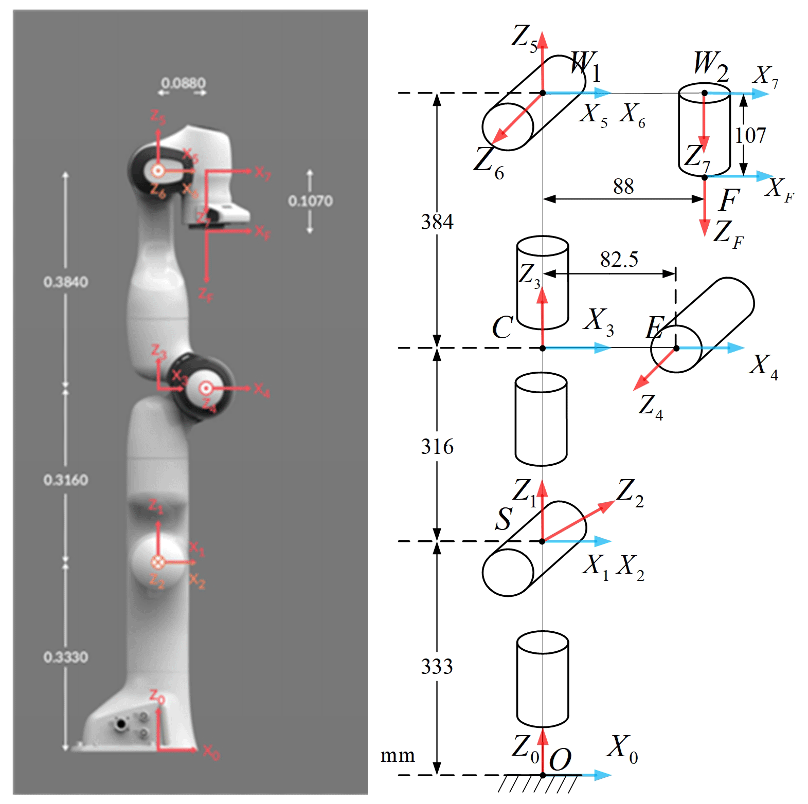
In this paper, the Franka–Emika robotic arm is studied for kinematic modeling according to the improved Denavit–Hartenberg (D-H) method, as shown in Fig. 4.

Figure 4 Robotic arm model and its simplified model.

Assume that the transformation matrix of coordinate systems between adjacent links is T and ⁱ⁻¹T_i denotes the transformation of the robot arm coordinate system {i} with respect to the coordinate system {i−1}. The general expression of ⁱ⁻¹T_i is as follows:

$$\begin{array}{}\text{(1)}& {}^{i-\mathrm{1}}{T}_i=\left[\begin{array}{cccc}c{\mathit{\theta }}_i& -s{\mathit{\theta }}_i& \mathrm{0}& a_{i-\mathrm{1}}\\ s{\mathit{\theta }}_{i}c{\mathit{\alpha }}_{i-\mathrm{2}}& c{\mathit{\theta }}_{i}c{\mathit{\alpha }}_{i-\mathrm{1}}& -s{\mathit{\alpha }}_{i-\mathrm{1}}& -s{\mathit{\alpha }}_{i-\mathrm{1}}{d}_i\\ s{\mathit{\theta }}_{i}s{\mathit{\alpha }}_{i-\mathrm{1}}& c{\mathit{\theta }}_{i}s{\mathit{\alpha }}_{i-\mathrm{1}}& c{\mathit{\alpha }}_{i-\mathrm{1}}& c{\mathit{\alpha }}_{i-\mathrm{1}}{d}_i\\ \mathrm{0}& \mathrm{0}& \mathrm{0}& \mathrm{1}\end{array}\right]\end{array}$$

$$\begin{array}{}\text{(2)}& {}^{\mathrm{0}}{T}_{\mathrm{F}}={}^{\mathrm{0}}{T}_{\mathrm{1}}\mathrm{\cdots }{}^{\mathrm{7}}{T}_{\mathrm{F}}=\left[\begin{array}{cccc}{n}_{mx}& o_{mx}& a_{mx}& p_{mx}\\ n_{my}& o_{my}& a_{my}& p_{my}\\ n_{mz}& o_{mz}& a_{mz}& p_{mz}\\ \mathrm{0}& \mathrm{0}& \mathrm{0}& \mathrm{1}\end{array}\right].\end{array}$$

3.1.2 Inverse kinematic analysis of robotic arm under RCM constraints

As can be seen from the robotic arm modeling, a₃ and a₄ are elbow bias, and a₆ is wrist bias, which does not meet the Piper criterion in robot kinematics. In this paper, the fixed-arm-shape angle parameter method is adopted to solve the inverse kinematics (Wang et al., 2022). When the pose ${}_F^{\mathrm{0}}T$ of the end effector is known, the joints of the robotic arm will rotate at a certain angle, as shown in Fig. 5.

Figure 5 Simplified model of the robot arm after rotating at a certain angle.

In ΔDSW₁, the equation can be obtained according to the law of cosine:

$$\begin{array}{}\text{(3)}& \cos {\mathit{\theta }}_{\mathrm{4}}={\displaystyle \frac{{∥{}^{\mathrm{0}}{L}_{s{w}_{\mathrm{1}}}∥}^{\mathrm{2}}-{∥SD∥}^{\mathrm{2}}-{∥W_{\mathrm{1}}D∥}^{\mathrm{2}}}{\mathrm{2}\cdot ∥SD∥\cdot ∥W_{\mathrm{1}}D∥}}\end{array}$$

$$\begin{array}{}\text{(4)}& {}^{\mathrm{0}}{T}_{\mathrm{6}}={}^{\mathrm{0}}{T}_{W\mathrm{1}}={}^{\mathrm{0}}{T}_{W\mathrm{2}}\cdot {}^{\mathrm{6}}{T}_{\mathrm{7}}^{-\mathrm{1}}=\left[\begin{array}{cc}{}^{\mathrm{0}}{R}_{\mathrm{6}}& {}^{\mathrm{0}}{P}_{\mathrm{6}}\\ \mathrm{0}& \mathrm{1}\end{array}\right]\end{array}$$

$$\begin{array}{}\text{(5)}& {}^{\mathrm{0}}{P}_{W\mathrm{1}}={}^{\mathrm{0}}{P}_{\mathrm{6}}.\end{array}$$

Here θ₇ is given in advance, and after the position of W₁ is obtained, the inverse kinematics solution of the manipulator can be obtained by the method of fixed-arm-shape Angle parameters. In this paper, the plane formed by points S, E and W₁ is called the arm plane. When θ₃=0, the plane formed by points O, S and W₁ is defined as the reference plane, and the arm angle φ is the angle between the arm plane and the reference plane, as shown in Fig. 6.

Figure 6 Definition of armature plane, reference plane and armature angle.

The actual motion of the robot arm can be seen as first reaching the target position in the reference plane and then rotating around the SW₁ axis by a certain angle.

$$\begin{array}{}\text{(6)}& {}^{\mathrm{0}}{R}_{\mathit{\phi }}=I_{\mathrm{3}}+\sin \mathit{\phi }\cdot \left[{}^{\mathrm{0}}{u}_{sw}\times \right]+\left(\mathrm{1}-\cos \mathit{\phi }\right)\cdot {\left[{}^{\mathrm{0}}{u}_{sw}\times \right]}^{\mathrm{2}}\end{array}$$

$$\begin{array}{}\text{(7)}& {}^{\mathrm{0}}{R}_k={}^{\mathrm{0}}{R}_{\mathit{\phi }}\cdot {}^{\mathrm{0}}{R}_k^{\mathrm{0}}\left(k=\mathrm{1},\mathrm{2}\mathrm{\dots }\mathrm{7}\right)\end{array}$$

$$\begin{array}{}\text{(8)}& {}^{\mathrm{0}}{L}_{S{W}_{\mathrm{1}}}={}^{\mathrm{0}}{R}_{\mathrm{3}}^{\mathrm{0}}\cdot {}^{\mathrm{3}}{L}_{S{W}_{\mathrm{1}}}\end{array}$$

$$\begin{array}{}\text{(9)}& {}^{\mathrm{0}}{R}_{\mathrm{3}}^{\mathrm{0}}=R\left({\mathit{\theta }}_{\mathrm{1}}^{\mathrm{0}}\right)\cdot R\left({\mathit{\theta }}_{\mathrm{2}}^{\mathrm{0}}\right)\cdot R\left({\mathit{\theta }}_{\mathrm{3}}^{\mathrm{0}}\right),\end{array}$$

where ${\mathit{\theta }}_{\mathrm{1}}^{\mathrm{0}}$, ${\mathit{\theta }}_{\mathrm{2}}^{\mathrm{0}}$ and ${\mathit{\theta }}_{\mathrm{3}}^{\mathrm{0}}$ denote the joint angle in the reference plane, while ${\mathit{\theta }}_{\mathrm{3}}^{\mathrm{0}}=\mathrm{0}$ and $R_{\mathrm{3}}^{\mathrm{0}}$ denote the rotation matrix in the reference plane.

$$\begin{array}{}\text{(10)}& {}^{\mathrm{0}}{R}_{\mathrm{3}}^{\mathrm{0}}=\left[\begin{array}{ccc}\cos {\mathit{\theta }}_{\mathrm{1}}^{\mathrm{0}}\cos {\mathit{\theta }}_{\mathrm{2}}^{\mathrm{0}}& -\sin {\mathit{\theta }}_{\mathrm{1}}^{\mathrm{0}}& \cos {\mathit{\theta }}_{\mathrm{1}}^{\mathrm{0}}\cos {\mathit{\theta }}_{\mathrm{2}}^{\mathrm{0}}\\ \sin {\mathit{\theta }}_{\mathrm{1}}^{\mathrm{0}}\cos {\mathit{\theta }}_{\mathrm{2}}^{\mathrm{0}}& \cos {\mathit{\theta }}_{\mathrm{1}}^{\mathrm{0}}& \sin {\mathit{\theta }}_{\mathrm{1}}^{\mathrm{0}}\sin {\mathit{\theta }}_{\mathrm{2}}^{\mathrm{0}}\\ -\sin {\mathit{\theta }}_{\mathrm{2}}^{\mathrm{0}}& \mathrm{0}& \cos {\mathit{\theta }}_{\mathrm{2}}^{\mathrm{0}}\end{array}\right]\end{array}$$

$$\begin{array}{}\text{(11)}& \left(-{}^{\mathrm{3}}{L}_{S{W}_{\mathrm{1}}}\left(\mathrm{1}\right)\right)\sin {\mathit{\theta }}_{\mathrm{2}}^{\mathrm{0}}+{}^{\mathrm{3}}{L}_{S{W}_{\mathrm{1}}}\left(\mathrm{3}\right)\cos {\mathit{\theta }}_{\mathrm{2}}^{\mathrm{0}}={}^{\mathrm{0}}{L}_{S{W}_{\mathrm{1}}}\left(\mathrm{3}\right)\end{array}$$

By solving the equation, one obtains ${\mathit{\theta }}_{\mathrm{2}}^{\mathrm{0}}$. Since the Y coordinate of the vector ${}^{\mathrm{3}}{L}_{S{W}_{\mathrm{1}}}$ is 0, the following equation can be obtained:

$$\begin{array}{}\text{(12)}& \sin {\mathit{\theta }}_{\mathrm{1}}^{\mathrm{0}}={\displaystyle \frac{{}^{\mathrm{0}}{L}_{S{W}_{\mathrm{1}}}\left(\mathrm{2}\right)}{{}^{\mathrm{3}}{L}_{S{W}_{\mathrm{1}}}\left(\mathrm{1}\right)\cos {\mathit{\theta }}_{\mathrm{2}}^{\mathrm{0}}+{}^{\mathrm{3}}{L}_{S{W}_{\mathrm{1}}}\left(\mathrm{3}\right)\sin {\mathit{\theta }}_{\mathrm{2}}^{\mathrm{0}}}}\end{array}$$

$$\begin{array}{}\text{(13)}& \cos {\mathit{\theta }}_{\mathrm{1}}^{\mathrm{0}}={\displaystyle \frac{{}^{\mathrm{0}}{L}_{S{W}_{\mathrm{1}}}\left(\mathrm{1}\right)}{{}^{\mathrm{3}}{L}_{S{W}_{\mathrm{1}}}\left(\mathrm{1}\right)\cos {\mathit{\theta }}_{\mathrm{2}}^{\mathrm{0}}+{}^{\mathrm{3}}{L}_{S{W}_{\mathrm{1}}}\left(\mathrm{3}\right)\sin {\mathit{\theta }}_{\mathrm{2}}^{\mathrm{0}}}}.\end{array}$$

At this point, ${\mathit{\theta }}_{\mathrm{1}}^{\mathrm{0}}$, ${\mathit{\theta }}_{\mathrm{2}}^{\mathrm{0}}$ and ${\mathit{\theta }}_{\mathrm{3}}^{\mathrm{0}}$ are known, and bringing them into Eq. (10) yields ${}^{\mathrm{0}}{R}_{\mathrm{3}}^{\mathrm{0}}$.

$$\begin{array}{}\text{(14)}& {}^{\mathrm{0}}{R}_{\mathrm{3}}={}^{\mathrm{0}}{R}_{\mathit{\phi }}\cdot {}^{\mathrm{0}}{R}_{\mathrm{3}}^{\mathrm{0}}\end{array}$$

$$\begin{array}{}\text{(15)}& {}^{\mathrm{0}}{R}_{\mathrm{3}}=As\cdot \sin \mathit{\phi }+Bs\cdot \cos \mathit{\phi }+Cs\end{array}$$

$$\begin{array}{}\text{(16)}& As=\left[{}^{\mathrm{0}}{u}_{sw}\times \right]{}^{\mathrm{0}}{R}_{\mathrm{3}}^{\mathrm{0}}\end{array}$$

$$\begin{array}{}\text{(17)}& Bs=-{\left[{{}^{\mathrm{0}}}_{sw}\times \right]}^{\mathrm{2}}{}^{\mathrm{0}}{R}_{\mathrm{3}}^{\mathrm{0}}\end{array}$$

$$\begin{array}{}\text{(18)}& Cs=\left[{}^{\mathrm{0}}{u}_{sw}^{\mathrm{0}}{u}_{sw}^T\right]{}^{\mathrm{0}}{R}_{\mathrm{3}}^{\mathrm{0}}\end{array}$$

$$\begin{array}{}\text{(19)}& {}^{\mathrm{0}}{R}_{\mathrm{3}}=\left[\begin{array}{ccc}\ast & \ast & \cos {\mathit{\theta }}_{\mathrm{1}}\sin {\mathit{\theta }}_{\mathrm{2}}\\ \ast & \ast & \sin {\mathit{\theta }}_{\mathrm{1}}\sin {\mathit{\theta }}_{\mathrm{2}}\\ -\sin {\mathit{\theta }}_{\mathrm{2}}\cos {\mathit{\theta }}_{\mathrm{3}}& \sin {\mathit{\theta }}_{\mathrm{2}}\sin {\mathit{\theta }}_{\mathrm{3}}& \cos {\mathit{\theta }}_{\mathrm{2}}\end{array}\right]\end{array}$$

$$\begin{array}{}\text{(20)}& \cos {\mathit{\theta }}_{\mathrm{2}}=A{s}_{\mathrm{33}}\sin \mathit{\phi }+B{s}_{\mathrm{33}}\cos \mathit{\phi }+C{s}_{\mathrm{33}}\end{array}$$

$$\begin{array}{}\text{(21)}& \sin {\mathit{\theta }}_{\mathrm{1}}={\displaystyle \frac{A{s}_{\mathrm{23}}\sin \mathit{\phi }+B{s}_{\mathrm{23}}\cos \mathit{\phi }+C{s}_{\mathrm{33}}}{\sin {\mathit{\theta }}_{\mathrm{2}}}}\end{array}$$

$$\begin{array}{}\text{(22)}& \cos {\mathit{\theta }}_{\mathrm{1}}={\displaystyle \frac{A{s}_{\mathrm{13}}\sin \mathit{\phi }+B{s}_{\mathrm{13}}\cos \mathit{\phi }+C{s}_{\mathrm{13}}}{\sin {\mathit{\theta }}_{\mathrm{2}}}}\end{array}$$

$$\begin{array}{}\text{(23)}& \sin {\mathit{\theta }}_{\mathrm{3}}={\displaystyle \frac{A{s}_{\mathrm{32}}\sin \mathit{\phi }+B{s}_{\mathrm{32}}\cos \mathit{\phi }+C{s}_{\mathrm{32}}}{\sin {\mathit{\theta }}_{\mathrm{2}}}}\end{array}$$

$$\begin{array}{}\text{(24)}& \cos {\mathit{\theta }}_{\mathrm{3}}={\displaystyle \frac{A{s}_{\mathrm{31}}\sin \mathit{\phi }+B{s}_{\mathrm{31}}\cos \mathit{\phi }+C{s}_{\mathrm{31}}}{-\sin {\mathit{\theta }}_{\mathrm{2}}}}\end{array}$$

$$\begin{array}{}\text{(25)}& {}^{\mathrm{4}}{R}_{\mathrm{7}}={\left({}^{\mathrm{3}}{R}_{\mathrm{3}}\right)}^T\cdot {\left({}^{\mathrm{0}}{R}_{\mathrm{4}}\right)}^T\cdot {}^{\mathrm{0}}{R}_{\mathrm{7}}\end{array}$$

Bringing Eq. (19) into Eq. (25),

$$\begin{array}{}\text{(26)}& {}^{\mathrm{4}}{R}_{\mathrm{7}}=Aw\cdot \sin \mathit{\phi }+Bw\cdot \cos \mathit{\phi }+Cw\end{array}$$

$$\begin{array}{}\text{(27)}& Aw={\left({}^{\mathrm{3}}{R}_{\mathrm{4}}\right)}^T\cdot A{\mathrm{s}}^T\cdot {}^{\mathrm{0}}{R}_{\mathrm{7}}\end{array}$$

$$\begin{array}{}\text{(28)}& Bw={\left({}^{\mathrm{3}}{R}_{\mathrm{4}}\right)}^T\cdot B{\mathrm{s}}^T\cdot {}^{\mathrm{0}}{R}_{\mathrm{7}}\end{array}$$

$$\begin{array}{}\text{(29)}& Cw={\left({}^{\mathrm{3}}{R}_{\mathrm{4}}\right)}^T\cdot C{\mathrm{s}}^T\cdot {}^{\mathrm{0}}{R}_{\mathrm{7}}\end{array}$$

$$\begin{array}{}\text{(30)}& {}^{\mathrm{4}}{R}_{\mathrm{7}}=\left[\begin{array}{ccc}\ast & \ast & \cos {\mathit{\theta }}_{\mathrm{5}}\sin {\mathit{\theta }}_{\mathrm{6}}\\ \sin {\mathit{\theta }}_{\mathrm{6}}\cos {\mathit{\theta }}_{\mathrm{7}}& -\sin {\mathit{\theta }}_{\mathrm{6}}\sin {\mathit{\theta }}_{\mathrm{7}}& -\cos {\mathit{\theta }}_{\mathrm{6}}\\ \ast & \ast & -\sin {\mathit{\theta }}_{\mathrm{5}}\sin {\mathit{\theta }}_{\mathrm{6}}\end{array}\right]\end{array}$$

$$\begin{array}{}\text{(31)}& \cos {\mathit{\theta }}_{\mathrm{6}}=-(A{w}_{\mathrm{23}}\sin \mathit{\phi }+B{w}_{\mathrm{23}}\cos \mathit{\phi }+C{w}_{\mathrm{23}})\end{array}$$

$$\begin{array}{}\text{(32)}& \sin {\mathit{\theta }}_{\mathrm{5}}={\displaystyle \frac{A{w}_{\mathrm{33}}\sin \mathit{\phi }+B{w}_{\mathrm{33}}\cos \mathit{\phi }+C{w}_{\mathrm{33}}}{-\sin {\mathit{\theta }}_{\mathrm{6}}}}\end{array}$$

$$\begin{array}{}\text{(33)}& \cos {\mathit{\theta }}_{\mathrm{5}}={\displaystyle \frac{A{w}_{\mathrm{13}}\sin \mathit{\phi }+B{w}_{\mathrm{13}}\cos \mathit{\phi }+C{w}_{\mathrm{13}}}{\sin {\mathit{\theta }}_{\mathrm{6}}}}\end{array}$$

$$\begin{array}{}\text{(34)}& \sin {\mathit{\theta }}_{\mathrm{7}}={\displaystyle \frac{A{w}_{\mathrm{22}}\sin \mathit{\phi }+B{w}_{\mathrm{22}}\cos \mathit{\phi }+C{w}_{\mathrm{22}}}{-\sin {\mathit{\theta }}_{\mathrm{6}}}}\end{array}$$

$$\begin{array}{}\text{(35)}& \cos {\mathit{\theta }}_{\mathrm{7}}={\displaystyle \frac{A{w}_{\mathrm{21}}\sin \mathit{\phi }+B{w}_{\mathrm{21}}\cos \mathit{\phi }+C{w}_{\mathrm{21}}}{\sin {\mathit{\theta }}_{\mathrm{6}}}}.\end{array}$$

The arm shape angle φ has a correspondence with the joint angle θ₇. When the joint angle θ₇ is given, the arm shape angle φ is also determined.

$$\begin{array}{}\text{(36)}& A\sin \mathit{\phi }+B\cos \mathit{\phi }+C=\mathrm{0}\end{array}$$

$$\begin{array}{}\text{(37)}& A=A{w}_{\mathrm{22}}+A{w}_{\mathrm{21}}\tan {\mathit{\theta }}_{\mathrm{7}}\end{array}$$

$$\begin{array}{}\text{(38)}& B=B{w}_{\mathrm{22}}+B{w}_{\mathrm{21}}\tan {\mathit{\theta }}_{\mathrm{7}}\end{array}$$

$$\begin{array}{}\text{(39)}& C=C{w}_{\mathrm{22}}+C{w}_{\mathrm{21}}\tan {\mathit{\theta }}_{\mathrm{7}}\end{array}$$

Applying the trigonometric constant transformations to the equations yields

$$\begin{array}{}\text{(40)}& \mathit{\phi }=\mathrm{atan}\mathrm{2}(-C,\pm \sqrt{A^{\mathrm{2}}+B^{\mathrm{2}}-C^{\mathrm{2}}})-\mathrm{atan}\mathrm{2}(B,A).\end{array}$$

The φ in Eq. (40) can be obtained by calculating and then substituting φ into the equation for all joint angles.

3.1.3 Kinematic verification of the robotic arm

The robot arm in this paper has a series rigid form, and the forward kinematics derivation and verification are relatively simple. The forward kinematics calculation results can be verified by inputting specific joint angles and comparing them with the real pose of the robot arm. This section mainly verifies the correctness of its inverse kinematics.

The basic process of the inverse kinematics verification of the manipulator is as follows: first, the forward and inverse kinematics function modules of the manipulator are established in the Simulink environment of MATLAB software. Secondly, given several joint angles within the limit of joint angles of the manipulator arm, the pose matrix of the end of the manipulator arm is calculated through forward kinematics, and the pose matrix is represented by position and Euler angle. Then the inverse solution of the pose matrix calculated by the forward kinematics is obtained, and the pose matrix is obtained by the forward kinematics and expressed by the position and Euler angle. Finally, the position obtained twice is compared with the Euler angle. If the results obtained twice are consistent, the correctness of the inverse kinematics can be verified.

Figure 7 Inverse kinematic simulation model.

The inverse kinematics simulation model of the manipulator is shown in Fig. 7. The position error obtained twice before and after is shown in Fig. 8a, and the Euler angle error is shown in Fig. 8b. Since MATLAB itself retains accuracy and effective floating point calculation, the calculation error of inverse kinematics can be considered to be 0 according to the order of magnitude of error of simulation results, thus verifying the correctness of inverse kinematics.

Figure 8 Kinematic inverse solution error.

3.2 Inverse kinematic analysis of the robot arm under RCM constraints

The end of the mechanical arm, the center of the telecentric fixed point and the target point are in the same line. The following formula can therefore be obtained:

$$\begin{array}{}\text{(41)}& p_{\mathrm{a}}=p_{\mathrm{t}}-{\displaystyle \frac{p_{\mathrm{t}}-p_{\mathrm{0}}}{∥p_{\mathrm{t}}-p_{\mathrm{0}}∥}}\cdot l.\end{array}$$

In Eq. (41), p_a is the end coordinate of the robotic arm, p_t is the target point coordinate, p₀ is the coordinates of the telecentric immobile point and l is the length from the end of the robotic arm to the end of the endoscope.

The orientation of the X and Y axes of the end coordinate system of the robot arm is irrelevant because the endoscope and the end Z axis are coaxial, which means that it only affects the angle of the seventh axis. After obtaining the angle of each joint of the robot arm, θ₇ is directly used as the joint angle of the seventh axis. The rotation matrix R of the end of the robot arm can be obtained by the equivalent rotation axis, and the end coordinate system Z axis can be written as

$$\begin{array}{}\text{(42)}& v_{\mathrm{e}}={\displaystyle \frac{p_{\mathrm{t}}-p_{\mathrm{0}}}{∥p_{\mathrm{t}}-p_{\mathrm{0}}∥}}.\end{array}$$

The Z axis of the robot arm base coordinate system can be written as

$$\begin{array}{}\text{(43)}& v_{\mathrm{b}}={\left[\mathrm{0},\mathrm{0},\mathrm{1}\right]}^T.\end{array}$$

Therefore, the equivalent rotation axis is

$$\begin{array}{}\text{(44)}& k=v_{\mathrm{e}}\times v_{\mathrm{b}}={\left[k_x{}^{\prime },k_y{}^{\prime },k_z{}^{\prime }\right]}^T.\end{array}$$

From the properties of the vector fork product of the above equation, k_z=0,

$$\begin{array}{}\text{(45)}& k=v_{\mathrm{e}}\times v_{\mathrm{b}}={\left[k_x,k_y,\mathrm{0}\right]}^T.\end{array}$$

$k_x=k_x{}^{\prime }/∥k{}^{\prime }∥,k_y=k_y{}^{\prime }/∥k{}^{\prime }∥$ in Eq. (45), and the equivalent rotation angle is

$$\begin{array}{}\text{(46)}& \mathit{\alpha }=\cos <v_{\mathrm{e}},v_{\mathrm{b}}>.\end{array}$$

According to the conversion relationship between the equivalent rotation axis and the rotation matrix, it can be obtained that

$$\begin{array}{}\text{(47)}& R=\left[\begin{array}{ccc}{k}_x{k}_x\mathrm{Vers}\mathit{\alpha }+c\mathit{\alpha }& k_x{k}_y\mathrm{Vers}\mathit{\alpha }& k_{y}s\mathit{\alpha }\\ k_x{k}_y\mathrm{Vers}\mathit{\alpha }& k_y{k}_y\mathrm{Vers}\mathit{\alpha }+c\mathit{\alpha }& -k_{x}s\mathit{\alpha }\\ -k_{y}s\mathit{\alpha }& k_{x}s\mathit{\alpha }& c\mathit{\alpha }\end{array}\right].\end{array}$$

In the above equation, $\mathrm{Vers}\mathit{\alpha }=\mathrm{1}-\cos \mathit{\alpha }$, and the end position of the robot arm is known. The robot arm inverse kinematics can be solved through the robot arm at each joint angle.

3.3 Flexible endoscopic robot trajectory planning experiment

The Franka robotic arm has seven joints. When the target position of each joint is known, this paper adopts closed-loop control based on joint position and joint velocity to realize the control of the robot arm. The following takes the single-joint controller as an example to introduce the overall design framework of the single-joint motion controller, including the position control, speed control and the kinematics, as shown in Fig. 9.

Figure 9 Overall design framework of single-joint motion controller for robotic arm.

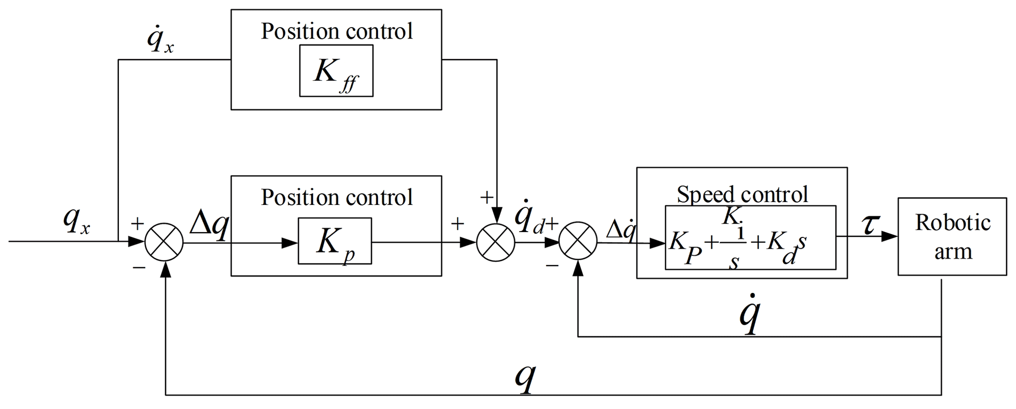
The single-joint motion controller consists of three parts: velocity feedforward control, position PID control and velocity PID control. The calculation formula of velocity feedforward control and position PID control is as follows:

$$\begin{array}{}\text{(48)}& {\dot{q}}_{\mathrm{d}}\left(t\right)=K_{\mathrm{p}}\left(q_x\left(t\right)-q\left(t\right)\right)+K_{\mathrm{ff}}{\dot{q}}_x\left(t\right).\end{array}$$

In Eq. (48), q_x is the desired position of the joint, q is the actual position of the joint, K_p is the proportionality coefficient, K_ff is the velocity feed-forward compensation coefficient and ${\dot{q}}_{\mathrm{d}}$ is the calculated desired velocity of the joint.

$$\begin{array}{}\text{(49)}& \begin{array}{ll}\mathit{\tau }\left(t\right)& =K_{\mathrm{p}}\mathrm{\Delta }\dot{q}\left(t\right)+K_{\mathrm{i}}\underset{\mathrm{0}}{\overset{t}{\int }}\mathrm{\Delta }\dot{q}\left(t\right)\mathrm{d}t+K_{\mathrm{d}}\mathrm{\Delta }\ddot{q}\left(t\right)\\ & =K_{\mathrm{p}}{\dot{q}}_{\mathrm{d}}\left(t\right)-\dot{q}\left(t\right)+K_{\mathrm{i}}\underset{\mathrm{0}}{\overset{t}{\int }}\left({\dot{q}}_{\mathrm{d}}\left(t\right)-\dot{q}\left(t\right)\right)\mathrm{d}t\\ & +K_{\mathrm{d}}\left({\ddot{q}}_{\mathrm{d}}\left(t\right)-\ddot{q}\left(t\right)\right)\end{array}\end{array}$$

In Eq. (49), K_p, K_i and K_d are the proportional, integral and differential coefficients; τ is the joint torque; and τ is the control signal passed to the robotic arm controller to control the joint motion of the robotic arm. PID closed-loop control can improve the response speed of the robot arm under the RCM constraint, which makes the robot arm movement more continuous and smoother, reducing the error at the RCM constraint point.

3.3.1 Verification of flexible endoscopic robot trajectory planning under RCM constraints

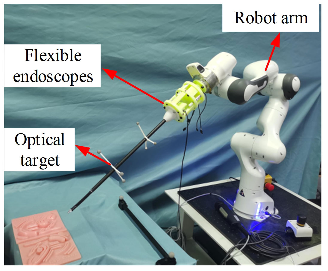
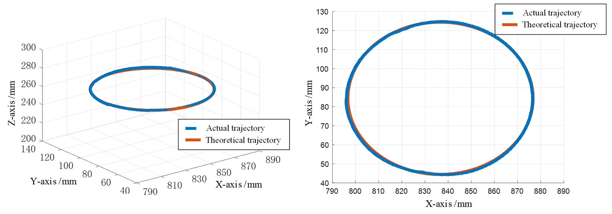
In order to verify the validity of kinematic analysis under RCM constraints, the experimental platform was firstly built as shown in Fig. 10, during which the RCM point position was recorded, and the flexible endoscope straight rod position was recorded in real time by installing an optical target point on the straight rod part of the flexible endoscope. Finally, the RCM error is calculated by calculating the distance from the RCM point to the straight line where the carbon fiber rod of the flexible endoscope is located, and the motion performance of the flexible endoscopic robot under the RCM constraint is evaluated. A set of circular trajectories with a radius of 40 mm is planned for the end of the flexible endoscopic robot. Compared with the linear or matrix trajectories, the circular trajectories are more complex, and the amplitude of the robot arm motion constraint is larger under the RCM, which has higher requirements on the control performance of the robot arm. The theoretical trajectory and the actual trajectory of the flexible endoscope robot are shown in Fig. 11.

Figure 10 Telecentric motionless point experimental platform.

Figure 11 Flexible endoscope trajectory comparison chart.

Figure 12 RCM error under motion capture system.

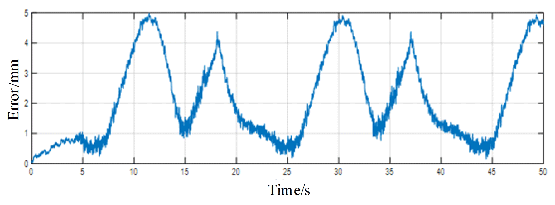
The experimental results are shown in Fig. 12, which is the error plot derived from the data recorded by the motion capture system. It can be seen that the error at the RCM constraint point is within 5 mm. In the real surgery, the position movement margin at the RCM point is about 10 mm, so it can be proved that the kinematic model based on the RCM point constraint adopted in this paper meets the surgery requirements.

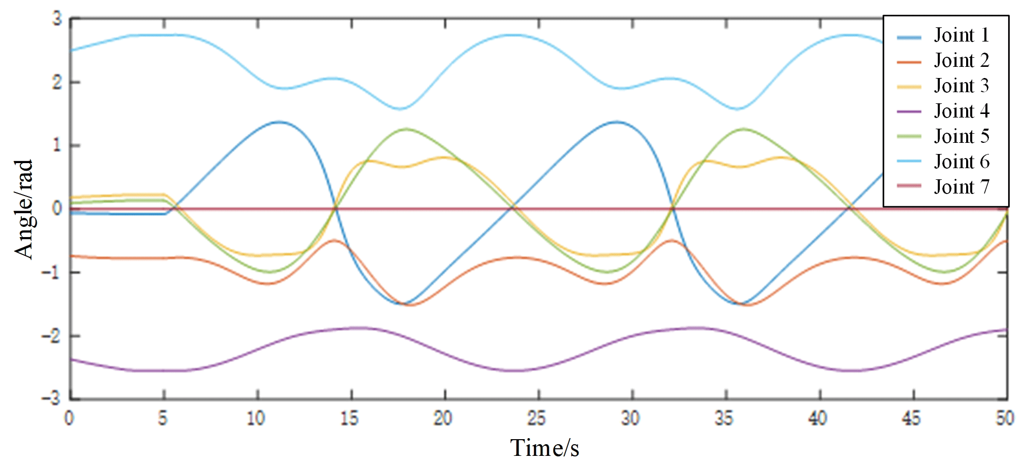
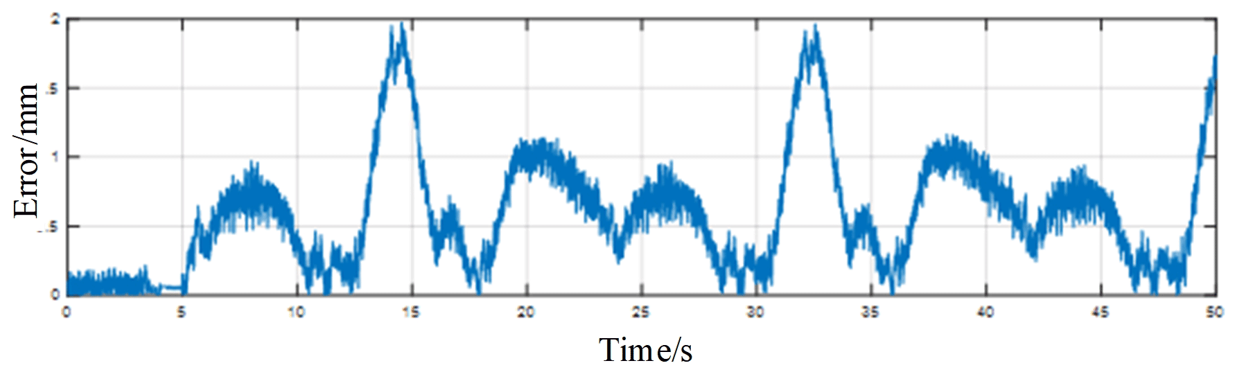
The reasons for the error at RCM constraint point are analyzed. One of the reasons is that the PID of the manipulator takes a certain time. Another reason is that the flexible endoscope system has errors during the 3D printing process and during assembly. Therefore, the data of each joint angle during the real-time movement of the robot arm are recorded during the experiment, as shown in Fig. 13. Each joint angle change during the real-time motion of the robot arm is periodic and free of vibration and shock, which is especially important for the safe and reliable operation of flexible endoscopic robots. Then the RCM point position and the flexible endoscope straight bar position are obtained through the positive kinematics of the robot arm, and finally the error of the RCM constraint point is calculated, as shown in Fig. 14. Experimental results show that the error of the RCM constraint point is less than 2 mm.

Figure 13 Data of each joint angle during the real-time movement of the robot arm.

Figure 14 RCM error under kinematic derivation.

3.4 Algorithm and experiment of heterogeneous primary–secondary teleoperation control based on position increments

The flexible endoscopic robot requires preoperative positioning before the surgical procedure, and the technique of primary–secondary teleoperation can help the surgeon to perform preoperative positioning and find the specific location of the lesion very well. Therefore, primary–secondary teleoperation has great application value in flexible endoscopic surgery. In this paper, the primary–secondary heterogeneous teleoperation control algorithm based on position increments is used to achieve the accurate control of the end of the flexible endoscopic robot through the method of proportional mapping.

3.4.1 Primary–secondary teleoperation control algorithm

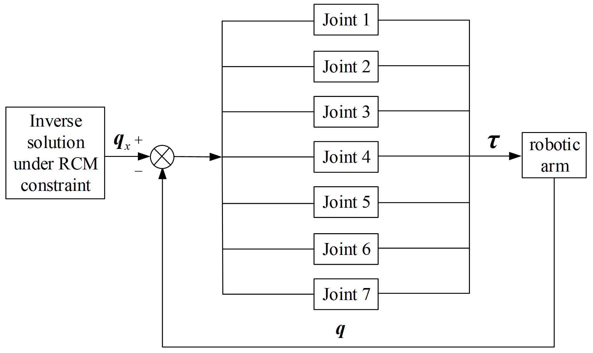
In this paper, the primary touch hand is used as the primary end device, and the secondary end is a flexible endoscopic robot. Meanwhile, the teleoperation should still be carried out under RCM constraints because the RCM constraint will produce hand–eye incoordination, which affects the quality of surgery. In order to solve the hand–eye coordination problem, the seventh joint of the robot arm is controlled alone (the seventh joint of the robot arm remains unchanged during the inverse solution). The block diagram of the teleoperation control under RCM constraints is shown in Fig. 15.

In the primary–secondary heterogeneous teleoperation control algorithm based on position increments, the zero position of the primary touch device is p_m0, and the zero position of the end of the flexible endoscope robot is p_s0. The zero point position of the end of the flexible endoscope robot is p_s0, which is not fixed and needs to be adjusted according to actual surgical requirements. The actual position of the main touch device is p_mc, and the actual position of the end of the flexible endoscope robot is p_sc. The primary–secondary mapping scheme based on location increments adopted in this paper is as follows:

$$\begin{array}{}\text{(50)}& p_{sc}=p_{s\mathrm{0}}+k(p_{mc}-p_{m\mathrm{0}}).\end{array}$$

The above formula indicates that the position increment of the current position of the primary device at a certain time relative to its zero position is (p_mc−p_m0). Considering the specific reasons such as primary–secondary heterogeneity and surgical application scenarios, it is necessary to multiply the scale factor k on the basis of the position increment to obtain the position increment of the secondary device relative to the zero position. At the same time, the mapping relationship between the joint angle of the main device and the seventh joint angle of the robot arm should also be multiplied by the corresponding proportional coefficient to ensure the safety of motion.

Figure 15 Primary–secondary remote operation control block diagram.

3.4.2 Primary–secondary teleoperation experiments and results

In order to test the primary–secondary tracking performance of the flexible endoscope robot, the following experiments are designed. The doctor operates the primary device to control the motion of the flexible endoscope robot and records the position information of the end of the endoscope robot. By comparing the theoretical position information recorded by the primary device with the actual end position information of the secondary endoscope robot, the primary–secondary three-dimensional space trajectory is drawn as shown in Fig. 16.

Figure 16 Primary–secondary track comparison chart.

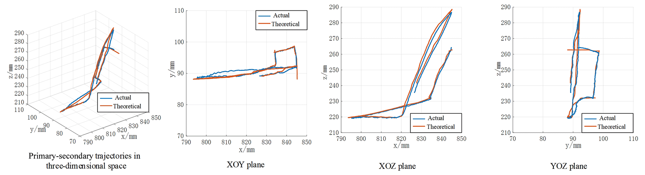
From Fig. 16, it can be seen that the flexible endoscopic robot can follow the specific position sent by the doctor for a good following motion, which can meet the basic requirements of the doctor. At the same time, the RCM constraint still has to be satisfied during the primary–secondary motion of the flexible endoscopic robot, and the RCM error is shown in Fig. 17 by specific calculation.

Figure 17 Primary–secondary RCM error plot.

4 Flexible endoscopic robot autonomous tracking experiment

Compared with traditional handheld endoscopic operations, introducing a flexible endoscopic robot to endoscopic surgery to provide the surgeon with a surgical field of view is a more intelligent and convenient solution. In order to achieve the position adjustment of the flexible endoscope robot according to the visual image information fed back by the endoscope, the position adjustment of the flexible endoscope robot ensures that the surgical instruments are always located in the center of the surgical field of view, so as to realize the function of autonomous tracking of surgical instruments. It specifically needs to meet the following two conditions: first, the flexible endoscope needs to identify different types of surgical instruments and obtain the corresponding position information, and, second, it then drives the endoscope to move through the real-time dynamic adjustment of the robot arm position, so as to obtain a good surgical field of view.

4.1 Deep learning target detection algorithm selection

For the processing of endoscopic visual information, this section focuses on the identification and positioning of surgical instruments. Traditional visual recognition and positioning methods, such as the use of markers for visual detection to achieve recognition, are not suitable for endoscopic surgery due to the risk of cross-infection in the actual surgical application, and the accuracy and speed do not meet the requirements. Through the analysis of the above requirements, and in order to quickly and accurately identify and locate surgical instruments in the actual application process, this section selects several current mainstream target detection algorithms to conduct relevant performance tests and conducts comparative analysis from the aspects of accuracy, recall rate and inference speed, so as to determine the final deep learning target detection algorithm.

4.1.1 Data set creation

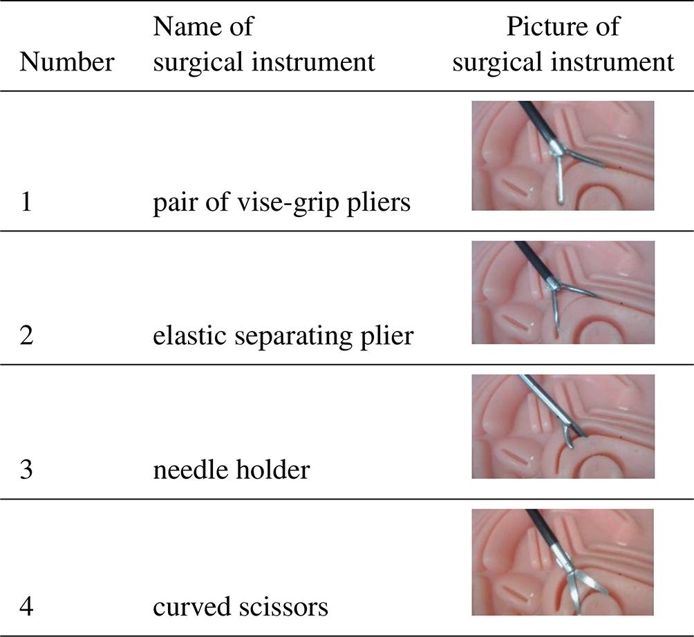
Due to the limited experimental conditions and the lack of real surgical materials in hospitals, this paper uses the Lap Game endoscopic surgery simulator as the data acquisition platform and selects several commonly used endoscopic surgical instruments. On this basis, with reference to the sampling and annotation methods of the relevant literature (Bawa et al., 2021, 2020), the relevant simulation surgery videos were recorded, and the images of different video frames were extracted at equal intervals through Python script files, which were used to evenly sample the image information of each stage of the surgery process, so as to obtain the endoscopic simulation surgery process data set. The relevant information is shown in Table 1.

Table 1 Categories of surgical instruments in the data set.

In order to obtain the accurate position of the end of the surgical instrument, this paper sorts each surgical instrument into two areas, namely the end part of the surgical instrument and the straight rod part of the surgical instrument. It includes the pixel center position of the region and the pixel size of the region, as shown in Fig. 18.

Figure 18 Surgical instrument end and straight rod labeling schematic.

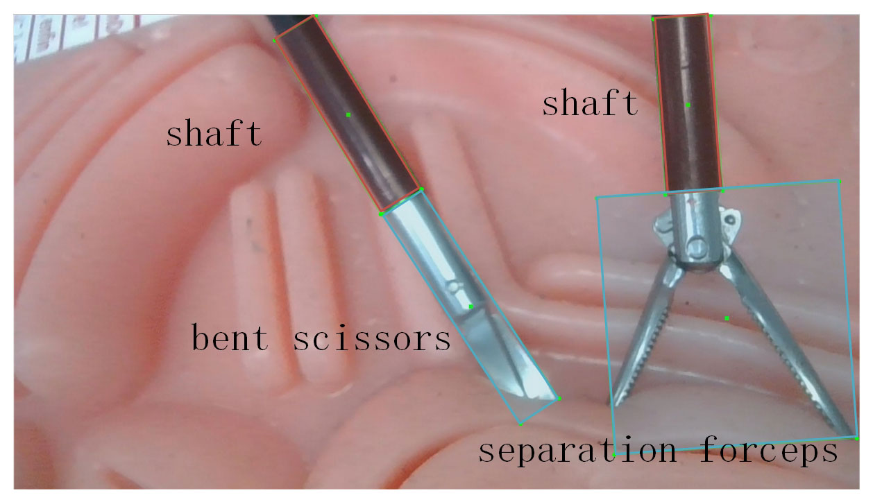
After the data set was made, the rotating annotation tool roLabelImg was used to annotate the data set, and a data set with 1000 pictures and 4000 annotations was finally established, among which 2000 were annotated on the end of surgical instruments, and 2000 were annotated on the straight rods of surgical instruments.

4.1.2 Comparison of deep learning target detection algorithms

Among the current mainstream deep learning target detection algorithms, three deep learning frameworks suitable for this paper, R3Det (Yang et al., 2021), Oriented R-CNN (Xie et al., 2021) and RTMDet (Lyu et al., 2022), are selected and compared and analyzed from several aspects.

Table 2 RTMDet model performance.

Table 3 Oriented R-CNN model performance.

Table 4 R3Det model performance.

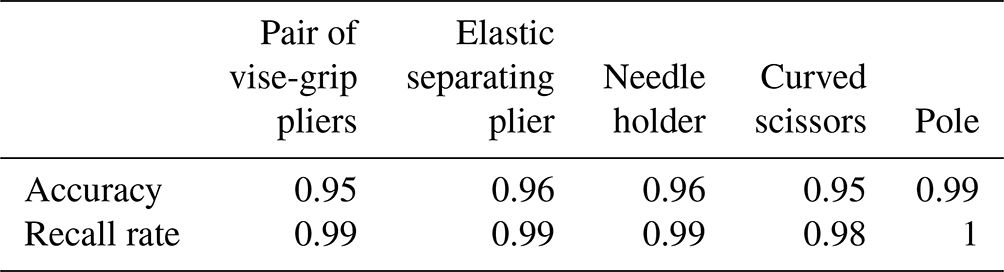
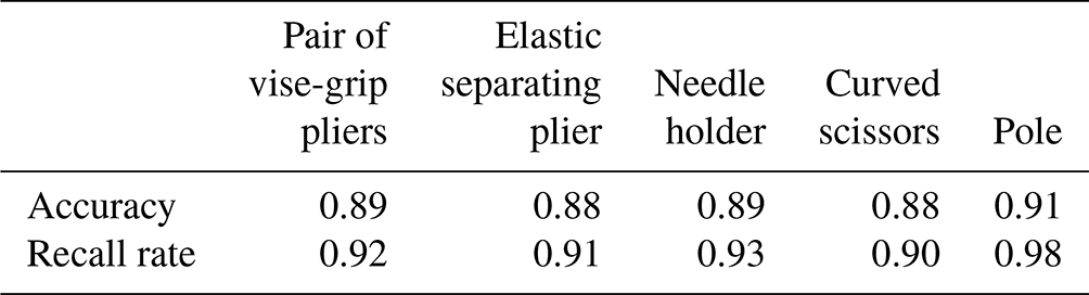
Comparing the three algorithms, RTMDet is far more effective than the other networks in terms of accuracy and recall. In addition to that, the inference speed of RTMDet is 10 fps (frame rate), which is much higher than that of the other two networks: Oriented E-CNN (5.91 fps), and R3Det (5.65 fps), and meets the demand of real-time tracking.

4.2 Autonomous tracking algorithm for flexible endoscopic robots

Here the center pixel of the surgical instrument detection box is marked as $p_{\mathrm{b}}=(u_{\mathrm{b}},v_{\mathrm{b}})$, and the center pixel of the image is marked as $p_{\mathrm{c}}=(u_{\mathrm{c}},v_{\mathrm{c}})$. The goal of autonomous tracking is to get p_b as close to the p_c as possible to get a good view. In order to accurately calculate the exact position of a surgical instrument under the endoscopic coordinate system, it is first necessary to calibrate the monocular endoscope with its internal reference matrix and hand–eye calibration matrix:

$$\begin{array}{}\text{(51)}& A=\left[\begin{array}{ccc}\frac{f}{d_x}& \mathrm{0}& u_{\mathrm{0}}\\ \mathrm{0}& \frac{f}{d_y}& v_{\mathrm{0}}\\ \mathrm{0}& \mathrm{0}& \mathrm{1}\end{array}\right]=\left[\begin{array}{ccc}\mathrm{1037.2}& \mathrm{0}& \mathrm{626.3}\\ \mathrm{0}& \mathrm{1001.9}& \mathrm{176.355}\\ \mathrm{0}& \mathrm{0}& \mathrm{1}\end{array}\right]\end{array}$$

$$\begin{array}{}\text{(52)}& \begin{array}{rl}{T}_b& =\left[\begin{array}{cc}R& t\\ \mathrm{0}& \mathrm{1}\end{array}\right]\\ & =\left[\begin{array}{cccc}-\mathrm{0.111}& -\mathrm{0.983}& -\mathrm{0.143}& \mathrm{5.636}\\ \mathrm{0.993}& -\mathrm{0.105}& -\mathrm{0.048}& \mathrm{6.372}\\ \mathrm{0.032}& -\mathrm{0.148}& \mathrm{0.989}& \mathrm{664.532}\\ \mathrm{0}& \mathrm{0}& \mathrm{0}& \mathrm{1}\end{array}\right].\end{array}\end{array}$$

Given the hand–eye calibration matrix above, the transformation relationship from the manipulator base coordinate system to the pixel coordinate system at a certain point in space can be obtained:

$$\begin{array}{}\text{(53)}& \begin{array}{rl}{Z}_c& \left[\begin{array}{c}u\\ v\\ \mathrm{1}\end{array}\right]=\left[\begin{array}{ccc}\frac{\mathrm{1}}{d_x}& \mathrm{0}& v_{\mathrm{0}}\\ \mathrm{0}& \frac{\mathrm{1}}{d_y}& u_{\mathrm{0}}\\ \mathrm{0}& \mathrm{0}& \mathrm{1}\end{array}\right]\\ & \left[\begin{array}{cccc}f& \mathrm{0}& \mathrm{0}& \mathrm{0}\\ \mathrm{0}& f& \mathrm{0}& \mathrm{0}\\ \mathrm{0}& \mathrm{0}& \mathrm{0}& \mathrm{0}\end{array}\right]\left[\begin{array}{cc}R& T\\ \mathrm{0}& \mathrm{1}\end{array}\right]\left[\begin{array}{c}{x}_w\\ y_w\\ z_w\\ \mathrm{1}\end{array}\right]\end{array}\end{array}$$

$$\begin{array}{}\text{(54)}& Z_c\left[\begin{array}{c}u\\ v\\ \mathrm{1}\end{array}\right]=M_C\cdot \left[R\mathrm{|}T\right]\cdot \left[\begin{array}{c}{x}_w\\ y_w\\ z_w\\ \mathrm{1}\end{array}\right]\end{array}$$

$$\begin{array}{}\text{(55)}& Z_c={\displaystyle \frac{f\cdot w}{p}}.\end{array}$$

In the above equation, Z_c is the depth information, f is the camera focal length, w is the width of the target object, and p is the pixel width of the target object in the picture. Similarly, the transformation relationship from the pixel coordinate system to the robot arm base coordinate system is expressed as

$$\begin{array}{}\text{(56)}& Z_c\cdot M_c^{-\mathrm{1}}\cdot \left[\begin{array}{c}u\\ v\\ \mathrm{1}\end{array}\right]=\left[R\mathrm{|}T\right]\cdot \left[\begin{array}{c}{x}_w\\ y_w\\ z_w\\ \mathrm{1}\end{array}\right]=R\cdot \left[\begin{array}{c}{x}_w\\ y_w\\ z_w\end{array}\right]+T\end{array}$$

$$\begin{array}{}\text{(57)}& \left[\begin{array}{c}{x}_w\\ y_w\\ z_w\end{array}\right]=R^{-\mathrm{1}}\cdot (M_c^{-\mathrm{1}}\cdot Z_c\cdot \left[\begin{array}{c}u\\ v\\ \mathrm{1}\end{array}\right]-T).\end{array}$$

It should be noted that [R|T] in the above equation is the external parameter matrix, which needs to be left-multiplied by the pose matrix T_a of the end of the manipulator in the robot base coordinate system on the basis of the hand–eye calibration matrix T_b. The coordinate of the end center of the surgical instrument in the base coordinate system of the robot arm is p_a2, the center coordinate of the camera field of vision is p_a1, the end coordinate of the flexible endoscope robot is p_t1 and the RCM point is p_o. It is assumed that the expected end coordinate of the flexible endoscope robot after adjustment is p_t2.

Using the similar geometric relationship in Fig. 19, it can be obtained that the movement vector of the end of the instrument arm in the base coordinate system of the robot arm is

$$\begin{array}{}\text{(58)}& {\displaystyle \frac{p_{t\mathrm{2}}-p_o}{p_{a\mathrm{2}}-p_o}}={\displaystyle \frac{d_{\mathrm{1}}}{d_{\mathrm{1}}+d_{\mathrm{2}}}}\text{(59)}& {\displaystyle }{p}_{t\mathrm{2}}={\displaystyle \frac{d_{\mathrm{1}}}{d_{\mathrm{1}}+d_{\mathrm{2}}}}\cdot \left(p_{a\mathrm{2}}-p_o\right)+p_o\text{(60)}& {\displaystyle }p=\mathit{\alpha }\cdot \left(p_{t\mathrm{2}}-p_{t\mathrm{1}}\right).\end{array}$$

Figure 19 Similar geometry schematic.

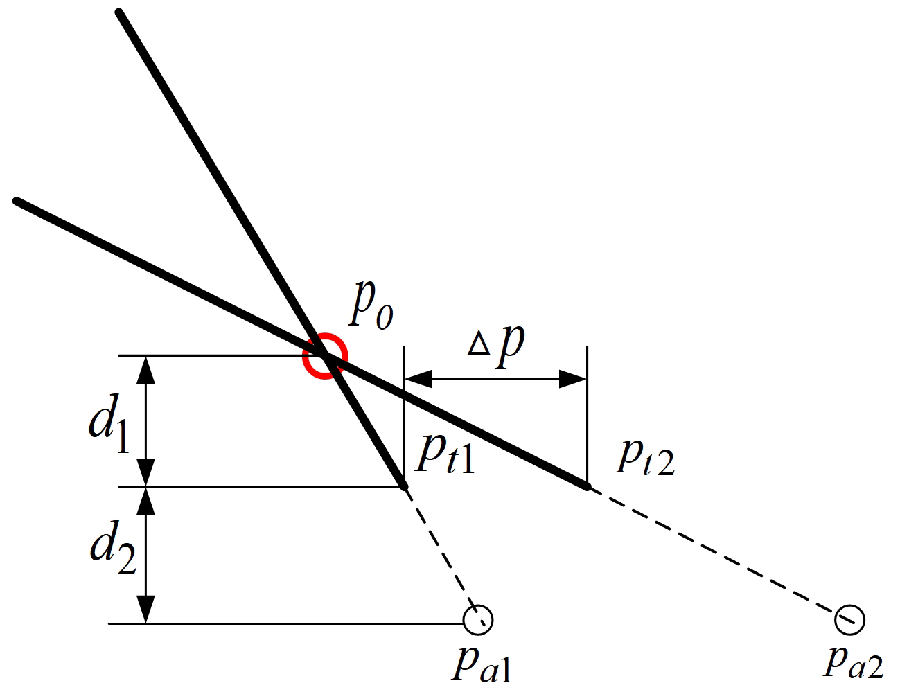
It should be explained that d₁ and d₂ are known in advance and remain unchanged in this article. Due to the large calibration error caused by the low pixel of the camera and the error of visual depth estimation, the above formula is essentially a proportional control method, in which the scale factor α determines the performance of the final tracking and realizes an autonomous tracking algorithm under specific conditions. The specific control framework is shown in the figure below.

Figure 20 Autonomous tracking algorithm control framework.

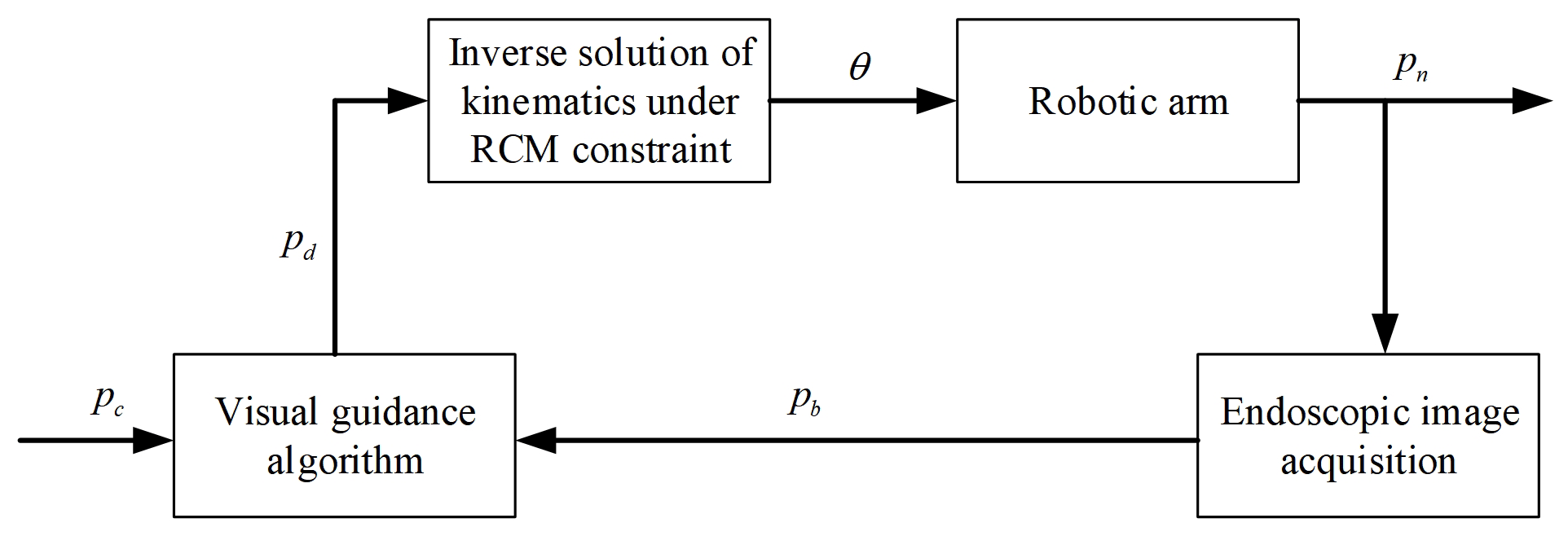
In the figure above, p_c is the target position of the surgical instrument center in the image, p_b is the current position of the surgical instrument center in the image, p_n is the current position of the end of the flexible endoscope robot and p_d is the target position of the end of the flexible endoscope robot.

4.3 Experimental study on autonomous tracking of flexible endoscopic robot

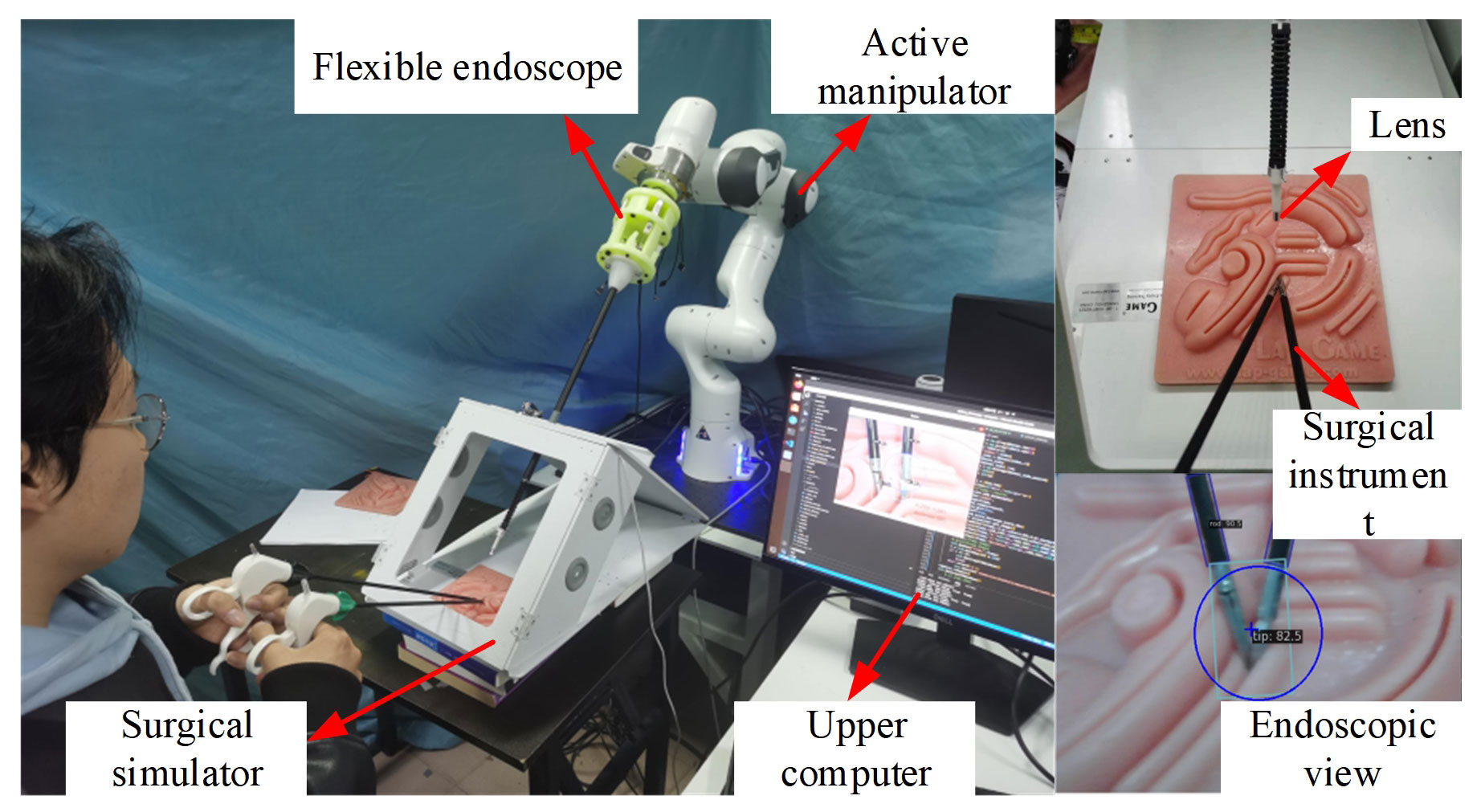
According to the analysis of common deep learning target detection models in the previous section, in the surgical instrument tracking experiment, the RTMDet algorithm was selected to generate the target recognition model, and the curved scissors and separation forceps were selected as experimental instruments. The pictures generated by the surgical simulator video were taken as the training set, and the strategy of marking the end of execution was adopted. A target recognition model is obtained which can return the center position coordinates of the detection frame in real time. Based on the motion control strategy introduced in the previous section, the simulation experiment platform as shown in Fig. 21 is built.

Figure 21 Overall picture of autonomous tracking experiment.

The experiment verifies that the motion control strategy proposed in this chapter can realize the control of the target surgical instrument to the center of the visual field under the guidance of the endoscopic image. As shown in Fig. 22, the central position of the end of the surgical instrument is gradually moved from both sides of the visual field to the center of the endoscopic visual field.

Figure 22 Visual field adjustment process.

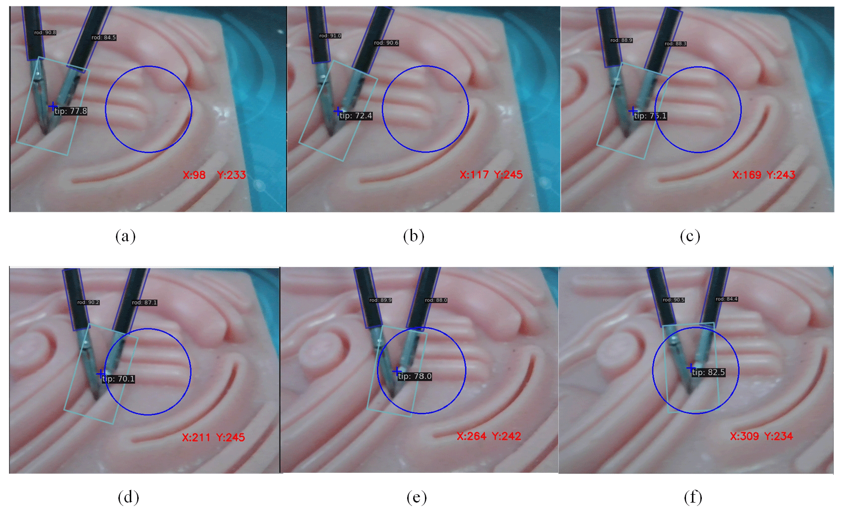
Meanwhile, in order to quantitatively describe the specific position of the central end position of the surgical instrument in the endoscopic visual field during the above visual field adjustment process, the coordinates of the central end position of the surgical instrument in the pixel coordinate system of the camera were recorded in real time in this section during the endoscopic autonomous tracking process, as shown in Fig. 23.

Figure 23 Field-of-view adjustment process pixel coordinates.

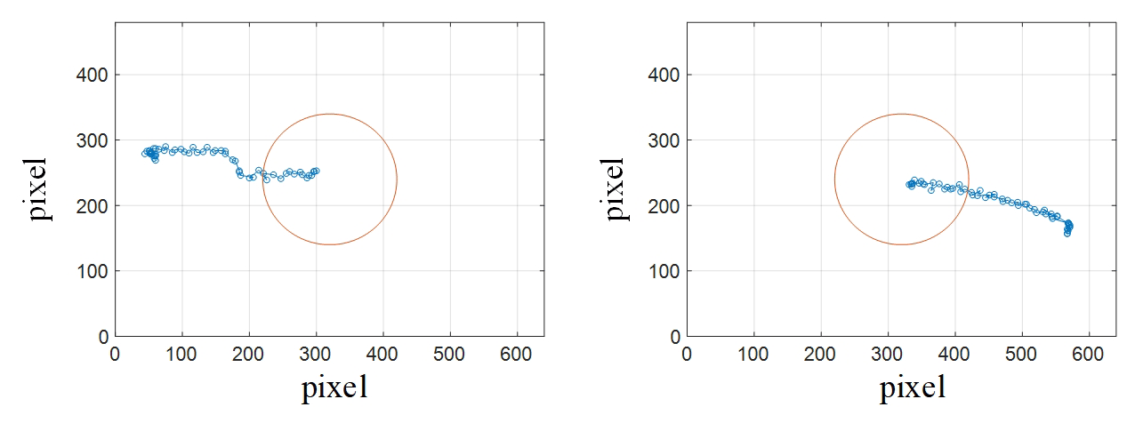
In Fig. 23, the available area of the endoscope's central field of vision is established with pixel coordinates (320, 240) as the center of the circle and 100 pixels as the radius, marked in red. As can be seen from Fig. 23, after adjusting the autonomous tracking strategy of the robotic arm, the central position of the end of the surgical instrument is in the central area of the endoscope field of view, which can provide doctors with a good surgical field of view and meet the surgical requirements.

Figure 24 Data of each joint angle during autonomous tracking motion.

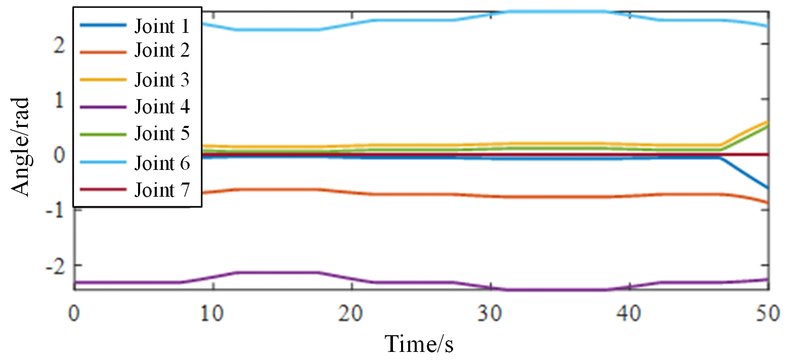
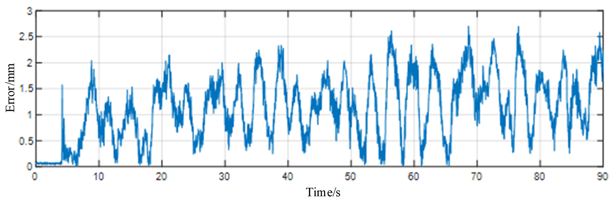
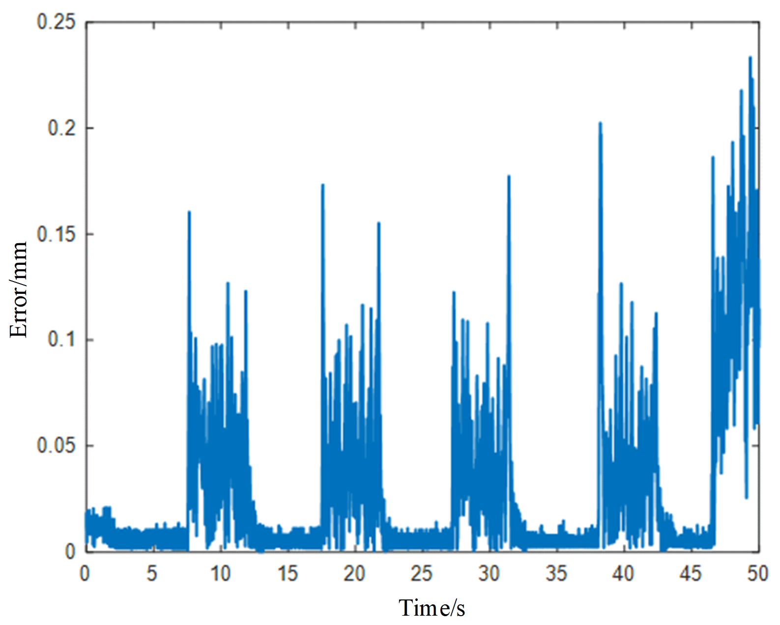
In order to further analyze the motion performance of the robot arm under the autonomous tracking control, this paper recorded the Angle data of each joint of the robot arm during the autonomous tracking process in real time and calculated the RCM error during the autonomous tracking process. As shown in Fig. 24, the data of each joint angle of the robotic arm change gently during autonomous tracking; the joint angle limitation is not exceeded, and there is no violent shaking phenomenon. As shown in Fig. 25, the RCM error during autonomous tracking is within 1 mm, which meets the requirements of real surgery and does not cause secondary trauma to the human body.

Figure 25 RCM error during autonomous tracking motion.

Through the analysis of the above experimental results, it can be seen that the data set established in this paper is convincing, and the deep learning object detection algorithm adopted can accurately and quickly complete the identification and positioning of surgical instruments. On this basis, the derived autonomous tracking control algorithm based on visual guidance can ensure that the center position of the surgical instrument is in the middle of the endoscopic field of view, and it can ensure a good RCM constraint effect during the autonomous tracking process.

5 Conclusions

The design of the flexible endoscopic robotic system is completed, and the key components of the flexible continuum joints are verified by finite element analysis and specific experiments to determine the optimal size. The constant curvature assumption method is used to model the kinematics of the 2-DOF flexible continuum, and the workspace of the flexible continuum is analyzed. Then, the kinematic calibration experiment is carried out on the continuum, and the kinematic model is calibrated by the method of drive compensation. The trajectory planning experiment was carried out with the calibrated kinematic model, and the functional verification of the flexible continuum was carried out to analyze the feasibility of its application in endoscopic surgery. Aiming at the RCM constraint problem during endoscopic surgery, the motion control algorithm of the flexible endoscopic robot under the RCM constraint was derived, and a set of circular trajectories with a radius of 40 mm was planned for its end, and the RCM error of the robotic arm in the process of motion, as well as the actual trajectory of the end of the continuum in the three-dimensional space, was obtained for the comparative analysis through the visual inspection system. Then a primary–secondary heterogeneous teleoperation control algorithm based on position increments was adopted to realize the precise control of the end of the flexible endoscopic robot by the method of proportional mapping. Finally, the RTMDet deep learning object detection algorithm was selected to identify and locate surgical instruments through comparative experiments, and the autonomous tracking control was completed based on visual guidance. In the process of autonomous tracking, the RCM error was less than 1 mm, which met the actual surgical requirements.