Stochastic stability and the moment Lyapunov exponent for a gyro-pendulum system driven by a bounded noise

The stochastic stability of a gyro-pendulum system parametrically excited by a real noise is investigated by the moment Lyapunov exponent in the paper. Using the spherical polar and non-singular linear stochastic transformations and combining these with Khasminskii's method, the diffusion process and the eigenvalue problem of the moment Lyapunov exponent are obtained. Then, applying the perturbation method and Fourier cosine series expansion, we derive an infinite-order matrix whose leading eigenvalue is the second-order expansion g₂(p) of the moment Lyapunov exponent. Thus, an infinite sequence for g₂(p) is constructed, and its convergence is numerically verified. Finally, the influences of the system and noise parameters on stochastic stability are given such that the stochastic stability is strengthened with the increased drift coefficient and the diffusion coefficient has the opposite effect; among the system parameters, only the increase in k and A₀ strengthens moment stability.

1 Introduction

There are many definitions of stochastic stability, among which the pth moment stability has attracted a lot of attention. The stability is usually described by the moment Lyapunov exponent, which was first presented in 1984 (Arnold, 1984). Then the moment Lyapunov exponent of the linear systems driven by the real and white noises was given, and the stochastic moment stability of linear system was completely resolved (Arnold et al., 1986a).

However, it is extremely difficult to obtain the analytic expression of the moment Lyapunov exponent for an actual dynamical system according to Arnold's results due to the complexity of the noise and system. So far, almost all the results about moment Lyapunov exponents were published through the approximate analytical methods. The asymptotic expansions of the moment Lyapunov exponents on a weak noise and a small value of p were first applied to analyse the stability of a two-dimensional stochastic system (Arnold et al., 1997). In a similar manner, Namachchivaya et al. (1996) studied the moment Lyapunov exponent for a system with two coupled oscillators excited by a real noise. For a linear conservative system with a white noise, Khasminskii and Moshchuk (1998) proved that both the moment Lyapunov exponent with the finite p and the stability index can only be regarded as the asymptotic expansions of small noise intensity. Referring to the results in a previous paper, for the same system and random excitation as Arnold et al. (1997), the asymptotic expansion of the finite pth moment Lyapunov exponent was also presented (Namachchivaya, 2001). For several two-dimensional systems with the real or bounded noise excitations, Xie (2001a, b, 2003) researched the weak noise expansions of the finite pth moment Lyapunov exponent, the maximal Lyapunov exponent, and the stability index through a similar procedure. The stability properties of a Van der Pol–Duffing oscillator excited by a real noise were investigated (Liu and Liew, 2005). Due to the complexity of approximate analytical methods, Higham et al. (2007) gave the numerical simulation of the moment Lyapunov exponent in stochastic differential equations. Then, the moment Lyapunov exponent and stochastic stability of a double-beam system under the compressive axial loading and moving narrow bands were discussed (Kozic et al., 2010). S. H. Li and X. B. Liu (2012, 2013) studied the moment Lyapunov exponent for a three-dimensional stochastic system based on the perturbation method. Hu et al. (2012, 2017) and X. Li and X. B. Liu (2013, 2014) obtained the moment Lyapunov exponent for a binary airfoil system under coloured noise excitation, which indicates stochastic dynamical theory has extended to the aviation field.

Gyro-pendulums are usually used to stabilise the firing of guns on warships or tanks or to navigate cars and aircraft, and the stability of the gyro-pendulum is a classical topic in dynamics and control, which made some researchers interested in it. The mean square and almost sure stability of a gyro-pendulum under random vertical support and white-noise excitation were researched through the stochastic averaging method (Namachchivaya, 1987; Asokanthan and Ariaratnam, 2000). Recently, the stochastic stability of a planner gyro-pendulum system excited by white noises has been presented (Li and Xu, 2019). However, as we know, the ideal white noise has infinite bandwidth and is difficult to achieve in practice. Therefore, we choose a bound noise to discuss the stochastic stability of a gyro-pendulum system parametrically driven by the bounded noise in this paper. In Sect. 2, the mathematical model is given. Applying a perturbation method, the eigenvalue problem of the moment Lyapunov exponent is obtained in Sect. 3 and solved via a Fourier cosine series expansion in Sect. 4. The numerical results are given in Sect. 5. In Sect. 6, the conclusions are presented.

2 Gyro-pendulum system excited by a bound noise

A typical gyro-pendulum system in the vertical configuration shown in Fig. 1 is considered, and its motion equations with a stochastic excitation f(t) are written as (Namachchivaya, 1987)

$$\begin{array}{}\text{(1)}& \begin{array}{l}{B}_{\mathrm{0}}{\ddot{\mathit{\theta }}}_{\mathrm{1}}+\text{Cn}{\dot{\mathit{\theta }}}_{\mathrm{2}}+\left[k+k_{\mathrm{1}}f\left(t\right)\right]{\mathit{\theta }}_{\mathrm{1}}=\mathrm{0},\\ A_{\mathrm{0}}{\ddot{\mathit{\theta }}}_{\mathrm{2}}-\text{Cn}{\dot{\mathit{\theta }}}_{\mathrm{1}}+\left[k+k_{\mathrm{1}}f\left(t\right)\right]{\mathit{\theta }}_{\mathrm{2}}=\mathrm{0},\end{array}\end{array}$$

where θ₁ and θ₂ are the motion of the outer gimbal about an inertial co-ordinate system OXYZ and the motion of the inner frame with respect to the y axis of the outer one, respectively. $A_{\mathrm{0}}=A+B^{\prime }$, $B_{\mathrm{0}}=A+A^{\prime }+A^{\prime \prime }$, A, and C are the inertial moment of the gyro about the rotation axis and any axis perpendicular to Oz. A^′ and B^′ are the inertial moments of the inner gimbal about the rotor principal axes Ox and Oy, respectively, and A^′′ represents the inertial moment of the outer frame about the axis OX. k=mgl denotes the pendulous stiffness, l is the pendulosity of the gyroscope, and n is the spin speed. k₁ is the stiffness of the excitation f(t).

Figure 1 A gyro-pendulum system in vertical configuration.

For the noise excitation, we introduce a bound noise cos [ξ(t)] because of its rather universal sense in engineering (Li and Wu, 2015; Li and Liu, 2012). Meanwhile, considering the system, damping the system Eq. (1) is rewritten as

$$\begin{array}{}\text{(2)}& \begin{array}{l}{\ddot{\mathit{\theta }}}_{\mathrm{1}}+{\mathit{\omega }}_{\mathrm{1}}^{\mathrm{2}}{\mathit{\theta }}_{\mathrm{1}}+{\mathit{\epsilon }}^{\mathrm{2}}\left(a_{\mathrm{11}}{\dot{\mathit{\theta }}}_{\mathrm{1}}+a_{\mathrm{12}}{\dot{\mathit{\theta }}}_{\mathrm{2}}\right)+\mathit{\epsilon }\left(b_{\mathrm{11}}{\mathit{\theta }}_{\mathrm{1}}+b_{\mathrm{12}}{\mathit{\theta }}_{\mathrm{2}}\right)\cos \left[\mathit{\xi }\right(t\left)\right]=\mathrm{0},\\ {\ddot{\mathit{\theta }}}_{\mathrm{2}}+{\mathit{\omega }}_{\mathrm{2}}^{\mathrm{2}}{\mathit{\theta }}_{\mathrm{2}}+{\mathit{\epsilon }}^{\mathrm{2}}\left(a_{\mathrm{21}}{\dot{\mathit{\theta }}}_{\mathrm{1}}+a_{\mathrm{22}}{\dot{\mathit{\theta }}}_{\mathrm{2}}\right)+\mathit{\epsilon }\left(b_{\mathrm{21}}{\mathit{\theta }}_{\mathrm{1}}+b_{\mathrm{22}}{\mathit{\theta }}_{\mathrm{2}}\right)\cos \left[\mathit{\xi }\right(t\left)\right]=\mathrm{0},\\ \mathrm{d}\mathit{\xi }\left(t\right)=\mathit{\mu }\mathrm{d}t+\mathit{\sigma }\circ \mathrm{d}W\left(t\right),\end{array}\end{array}$$

where $\mathrm{0}<\mathit{\epsilon }\ll \mathrm{1}$ is a very small number. ${\mathit{\omega }}_{\mathrm{1}}^{\mathrm{2}}=k/B_{\mathrm{0}}$, ${\mathit{\omega }}_{\mathrm{2}}^{\mathrm{2}}=k/A_{\mathrm{0}}$, a₁₁=d₂/B₀, a₁₂=Cn/B₀, $a_{\mathrm{21}}=-\text{Cn}/A_{\mathrm{0}}$, a₂₂=d₁/A₀, d₁, and d₂ are damping coefficients. $b_{\mathrm{11}}=b_{\mathrm{12}}=k_{\mathrm{1}}/B_{\mathrm{0}}$; $b_{\mathrm{21}}=b_{\mathrm{22}}=k_{\mathrm{1}}/A_{\mathrm{0}}$. The symbol “∘” represents that Eq. (2) is a Stratonovich stochastic differential equation, μ is drift coefficient, σ is diffusion coefficient, and both are any real constants; W(t) is a unit Wiener process.

Letting θ₁=x₁, ${\dot{\mathit{\theta }}}_{\mathrm{1}}={\mathit{\omega }}_{\mathrm{1}}{x}_{\mathrm{2}}$, θ₂=x₃, and ${\dot{\mathit{\theta }}}_{\mathrm{2}}={\mathit{\omega }}_{\mathrm{2}}{x}_{\mathrm{4}}$, Eq. (2) is changed into a vector-matrix equation:

$$\begin{array}{}\text{(3)}& \left\{\begin{array}{l}\dot{\mathit{x}}=\left({\mathbf{A}}_{\mathrm{0}}+{\mathit{\epsilon }}^{\mathrm{2}}{\mathbf{A}}_{\mathrm{1}}\right)\mathit{x}+\mathit{\epsilon }\cos \left(\mathit{\xi }\right(t\left)\right)\mathbf{B}\mathit{x}\\ \mathrm{d}\mathit{\xi }\left(t\right)=\mathit{\mu }\mathrm{d}t+\mathit{\sigma }\circ \mathrm{d}W\left(t\right).\end{array}\right.\end{array}$$

where

$$\begin{array}{rl}& {\mathbf{A}}_{\mathrm{0}}=\left[\begin{array}{cccc}\mathrm{0}& {\mathit{\omega }}_{\mathrm{1}}& \mathrm{0}& \mathrm{0}\\ -{\mathit{\omega }}_{\mathrm{1}}& \mathrm{0}& \mathrm{0}& \mathrm{0}\\ \mathrm{0}& \mathrm{0}& \mathrm{0}& {\mathit{\omega }}_{\mathrm{2}}\\ \mathrm{0}& \mathrm{0}& -{\mathit{\omega }}_{\mathrm{2}}& \mathrm{0}\end{array}\right],\\ & {\mathbf{A}}_{\mathrm{1}}=\left[\begin{array}{cccc}\mathrm{0}& \mathrm{0}& \mathrm{0}& \mathrm{0}\\ \mathrm{0}& -a_{\mathrm{11}}& \mathrm{0}& -\frac{{\mathit{\omega }}_{\mathrm{2}}{a}_{\mathrm{12}}}{{\mathit{\omega }}_{\mathrm{1}}}\\ \mathrm{0}& \mathrm{0}& \mathrm{0}& \mathrm{0}\\ \mathrm{0}& -\frac{{\mathit{\omega }}_{\mathrm{1}}{a}_{\mathrm{21}}}{{\mathit{\omega }}_{\mathrm{2}}}& \mathrm{0}& -a_{\mathrm{22}}\end{array}\right],\\ & \mathbf{B}=\left[\begin{array}{cccc}\mathrm{0}& \mathrm{0}& \mathrm{0}& \mathrm{0}\\ -\frac{b_{\mathrm{11}}}{{\mathit{\omega }}_{\mathrm{1}}}& \mathrm{0}& -\frac{b_{\mathrm{12}}}{{\mathit{\omega }}_{\mathrm{1}}}& \mathrm{0}\\ \mathrm{0}& \mathrm{0}& \mathrm{0}& \mathrm{0}\\ -\frac{b_{\mathrm{21}}}{{\mathit{\omega }}_{\mathrm{2}}}& \mathrm{0}& -\frac{b_{\mathrm{22}}}{{\mathit{\omega }}_{\mathrm{2}}}& \mathrm{0}\end{array}\right].\end{array}$$

Through applying the spherical polar transformation

$$\begin{array}{rl}& x_{\mathrm{1}}=\mathit{\rho }\cos {\mathit{\phi }}_{\mathrm{1}}\cos \mathit{\theta },x_{\mathrm{2}}=-\mathit{\rho }\sin {\mathit{\phi }}_{\mathrm{1}}\cos \mathit{\theta },\\ & x_{\mathrm{3}}=-\mathit{\rho }\cos {\mathit{\phi }}_{\mathrm{2}}\sin \mathit{\theta },x_{\mathrm{4}}=-\mathit{\rho }\sin {\mathit{\phi }}_{\mathrm{2}}\sin \mathit{\theta },\\ & P={∥X∥}^p={\mathit{\rho }}^p,{\mathit{\phi }}_{\mathrm{1}},{\mathit{\phi }}_{\mathrm{2}}\in \left[\mathrm{0},\mathrm{2}\mathit{\pi }\right],\mathit{\theta }\in \left[-\mathit{\pi }/\mathrm{2},\mathit{\pi }/\mathrm{2}\right],\end{array}$$

and substituting them into Eq. (3), the equations for norm process P and phase processes θ, ϕ₁, and ϕ₂ can be obtained according to Itô's lemma:

$$\begin{array}{}\text{(4)}& \begin{array}{l}\dot{P}=\mathit{\epsilon }p{\mathit{\rho }}_{\mathrm{1}}P\cos \left[\mathit{\xi }\right(t\left)\right]+{\mathit{\epsilon }}^{\mathrm{2}}p{\mathit{\rho }}_{\mathrm{2}}P,\\ \dot{\mathit{\theta }}=\mathit{\epsilon }{\mathit{\theta }}_{\mathrm{1}}\cos \left[\mathit{\xi }\right(t\left)\right]+{\mathit{\epsilon }}^{\mathrm{2}}{\mathit{\theta }}_{\mathrm{2}},\\ {\dot{\mathit{\phi }}}_{\mathrm{1}}={\mathit{\omega }}_{\mathrm{1}}+\mathit{\epsilon }{\mathit{\phi }}_{\mathrm{11}}\cos \left[\mathit{\xi }\right(t\left)\right]+{\mathit{\epsilon }}^{\mathrm{2}}{\mathit{\phi }}_{\mathrm{12}},\\ {\dot{\mathit{\phi }}}_{\mathrm{2}}={\mathit{\omega }}_{\mathrm{2}}+\mathit{\epsilon }{\mathit{\phi }}_{\mathrm{21}}\cos \left[\mathit{\xi }\right(t\left)\right]+{\mathit{\epsilon }}^{\mathrm{2}}{\mathit{\phi }}_{\mathrm{22}},\\ \mathrm{d}\mathit{\xi }\left(t\right)=\mathit{\mu }\mathrm{d}t+\mathit{\sigma }\mathrm{d}W\left(t\right),\end{array}\end{array}$$

where

$$\begin{array}{rl}{\mathit{\rho }}_{\mathrm{1}}& ={\displaystyle \frac{\mathrm{1}}{\mathrm{2}{\mathit{\omega }}_{\mathrm{1}}}}\left[b_{\mathrm{11}}\sin \left(\mathrm{2}{\mathit{\phi }}_{\mathrm{1}}\right){\cos }^{\mathrm{2}}\left(\mathit{\theta }\right)+b_{\mathrm{12}}\sin \left({\mathit{\phi }}_{\mathrm{1}}\right)\cos \left({\mathit{\phi }}_{\mathrm{2}}\right)\sin \left(\mathrm{2}\mathit{\theta }\right)\right],\\ & +{\displaystyle \frac{\mathrm{1}}{\mathrm{2}{\mathit{\omega }}_{\mathrm{2}}}}\left[b_{\mathrm{21}}\sin \left({\mathit{\phi }}_{\mathrm{2}}\right)\cos \left({\mathit{\phi }}_{\mathrm{1}}\right)\sin \left(\mathrm{2}\mathit{\theta }\right)+b_{\mathrm{22}}\sin \left(\mathrm{2}{\mathit{\phi }}_{\mathrm{2}}\right){\sin }^{\mathrm{2}}\left(\mathit{\theta }\right)\right]\end{array},$$

$$\begin{array}{rl}{\mathit{\rho }}_{\mathrm{2}}& =-\left[a_{\mathrm{11}}{\sin }^{\mathrm{2}}\left({\mathit{\phi }}_{\mathrm{1}}\right){\cos }^{\mathrm{2}}\left(\mathit{\theta }\right)+a_{\mathrm{22}}{\sin }^{\mathrm{2}}\left({\mathit{\phi }}_{\mathrm{2}}\right){\sin }^{\mathrm{2}}\left(\mathit{\theta }\right)\right],\\ & -{\displaystyle \frac{\mathrm{1}}{\mathrm{2}}}\left({\displaystyle \frac{{\mathit{\omega }}_{\mathrm{2}}{a}_{\mathrm{12}}}{{\mathit{\omega }}_{\mathrm{1}}}}+{\displaystyle \frac{{\mathit{\omega }}_{\mathrm{1}}{a}_{\mathrm{21}}}{{\mathit{\omega }}_{\mathrm{2}}}}\right)\sin \left({\mathit{\phi }}_{\mathrm{1}}\right)\cos \left({\mathit{\phi }}_{\mathrm{2}}\right)\sin \left(\mathrm{2}\mathit{\theta }\right),\end{array}$$

$$\begin{array}{rl}{\mathit{\theta }}_{\mathrm{1}}& ={\displaystyle \frac{\mathrm{1}}{\mathrm{4}}}\left[{\displaystyle \frac{b_{\mathrm{22}}}{{\mathit{\omega }}_{\mathrm{2}}}}\sin \left(\mathrm{2}{\mathit{\phi }}_{\mathrm{2}}\right)-{\displaystyle \frac{b_{\mathrm{11}}}{{\mathit{\omega }}_{\mathrm{1}}}}\sin \left(\mathrm{2}{\mathit{\phi }}_{\mathrm{1}}\right)\right]\sin \left(\mathrm{2}\mathit{\theta }\right),\\ & +{\displaystyle \frac{b_{\mathrm{21}}}{{\mathit{\omega }}_{\mathrm{2}}}}\sin \left({\mathit{\phi }}_{\mathrm{2}}\right)\cos \left({\mathit{\phi }}_{\mathrm{1}}\right){\cos }^{\mathrm{2}}\left(\mathit{\theta }\right)-{\displaystyle \frac{b_{\mathrm{12}}}{{\mathit{\omega }}_{\mathrm{1}}}}\sin \left({\mathit{\phi }}_{\mathrm{1}}\right)\cos \left({\mathit{\phi }}_{\mathrm{2}}\right){\sin }^{\mathrm{2}}\left(\mathit{\theta }\right),\end{array}$$

$$\begin{array}{rl}{\mathit{\theta }}_{\mathrm{2}}& ={\displaystyle \frac{\mathrm{1}}{\mathrm{2}}}\left[a_{\mathrm{11}}{\sin }^{\mathrm{2}}\left({\mathit{\phi }}_{\mathrm{1}}\right)-a_{\mathrm{22}}{\sin }^{\mathrm{2}}\left({\mathit{\phi }}_{\mathrm{2}}\right)\right]\sin \left(\mathrm{2}\mathit{\theta }\right),\\ & +\left[{\displaystyle \frac{{\mathit{\omega }}_{\mathrm{2}}{a}_{\mathrm{12}}}{{\mathit{\omega }}_{\mathrm{1}}}}{\sin }^{\mathrm{2}}\left(\mathit{\theta }\right)-{\displaystyle \frac{{\mathit{\omega }}_{\mathrm{1}}{a}_{\mathrm{21}}}{{\mathit{\omega }}_{\mathrm{2}}}}{\cos }^{\mathrm{2}}\left(\mathit{\theta }\right)\right]\sin \left({\mathit{\phi }}_{\mathrm{1}}\right)\sin \left({\mathit{\phi }}_{\mathrm{2}}\right),\end{array}$$

$${\mathit{\phi }}_{\mathrm{11}}={\displaystyle \frac{\mathrm{1}}{{\mathit{\omega }}_{\mathrm{1}}}}\left[b_{\mathrm{11}}{\cos }^{\mathrm{2}}\left({\mathit{\phi }}_{\mathrm{1}}\right)+b_{\mathrm{12}}\cos \left({\mathit{\phi }}_{\mathrm{1}}\right)\cos \left({\mathit{\phi }}_{\mathrm{2}}\right)\tan \left(\mathit{\theta }\right)\right],$$

$${\mathit{\phi }}_{\mathrm{12}}=-\left[{\displaystyle \frac{a_{\mathrm{11}}}{\mathrm{2}}}\sin \left(\mathrm{2}{\mathit{\phi }}_{\mathrm{1}}\right)+{\displaystyle \frac{{\mathit{\omega }}_{\mathrm{2}}{a}_{\mathrm{12}}}{{\mathit{\omega }}_{\mathrm{1}}}}\sin \left({\mathit{\phi }}_{\mathrm{2}}\right)\cos \left({\mathit{\phi }}_{\mathrm{1}}\right)\tan \left(\mathit{\theta }\right)\right],$$

$${\mathit{\phi }}_{\mathrm{21}}={\displaystyle \frac{\mathrm{1}}{{\mathit{\omega }}_{\mathrm{2}}}}\left[b_{\mathrm{21}}\cos \left({\mathit{\phi }}_{\mathrm{1}}\right)\cos \left({\mathit{\phi }}_{\mathrm{2}}\right)\cot \left(\mathit{\theta }\right)+b_{\mathrm{22}}{\cos }^{\mathrm{2}}\left({\mathit{\phi }}_{\mathrm{2}}\right)\right],$$

$${\mathit{\phi }}_{\mathrm{22}}=-\left[{\displaystyle \frac{a_{\mathrm{11}}}{\mathrm{2}}}\sin \left(\mathrm{2}{\mathit{\phi }}_{\mathrm{2}}\right)+{\displaystyle \frac{{\mathit{\omega }}_{\mathrm{1}}{a}_{\mathrm{21}}}{{\mathit{\omega }}_{\mathrm{2}}}}\sin \left({\mathit{\phi }}_{\mathrm{1}}\right)\cos \left({\mathit{\phi }}_{\mathrm{2}}\right)\cot \left(\mathit{\theta }\right)\right].$$

For the norm process P, a non-singular linear stochastic transformation is introduced, i.e.

$$\begin{array}{}\text{(5)}& \begin{array}{rl}& S=T\left(\mathit{\theta },{\mathit{\phi }}_{\mathrm{1}},{\mathit{\phi }}_{\mathrm{2}},\mathit{\xi }\right)P,P=T^{-\mathrm{1}}\left(\mathit{\theta },{\mathit{\phi }}_{\mathrm{1}},{\mathit{\phi }}_{\mathrm{2}},\mathit{\xi }\right)S,\\ & \mathrm{0}\le \mathit{\theta }\le \mathit{\pi }/\mathrm{2},\mathrm{0}\le {\mathit{\phi }}_{\mathrm{1}},{\mathit{\phi }}_{\mathrm{2}},\mathit{\xi }\le \mathrm{2}\mathit{\pi },\end{array}\end{array}$$

where the function $T\left(\mathit{\theta },{\mathit{\phi }}_{\mathrm{1}},{\mathit{\phi }}_{\mathrm{2}},\mathit{\xi }\right)$ is a scalar function of the phase processes $\left(\mathit{\theta },{\mathit{\phi }}_{\mathrm{1}},{\mathit{\phi }}_{\mathrm{2}},\mathit{\xi }\right)$. Thus, Itô's stochastic equation for the new norm process S is derived by Itô's lemma:

$$\begin{array}{}\text{(6)}& \begin{array}{rl}\mathrm{d}S& =P[\mathit{\mu }{\displaystyle \frac{\partial }{\partial \mathit{\xi }}}+{\displaystyle \frac{\mathrm{1}}{\mathrm{2}}}{\mathit{\sigma }}^{\mathrm{2}}{\displaystyle \frac{{\partial }^{\mathrm{2}}}{\partial {\mathit{\xi }}^{\mathrm{2}}}}+{\mathit{\omega }}_{\mathrm{1}}{\displaystyle \frac{\partial }{\partial {\mathit{\phi }}_{\mathrm{1}}}}+{\mathit{\omega }}_{\mathrm{2}}{\displaystyle \frac{\partial }{\partial {\mathit{\phi }}_{\mathrm{2}}}}\\ & +\mathit{\epsilon }\left(p{\mathit{\rho }}_{\mathrm{1}}+{\mathit{\theta }}_{\mathrm{1}}{\displaystyle \frac{\partial }{\partial \mathit{\theta }}}+{\mathit{\phi }}_{\mathrm{11}}{\displaystyle \frac{\partial }{\partial {\mathit{\phi }}_{\mathrm{1}}}}+{\mathit{\phi }}_{\mathrm{21}}{\displaystyle \frac{\partial }{\partial {\mathit{\phi }}_{\mathrm{2}}}}\right)\cos \left(\mathit{\xi }\right)\\ & +{\mathit{\epsilon }}^{\mathrm{2}}\left(p{\mathit{\rho }}_{\mathrm{2}}+{\mathit{\theta }}_{\mathrm{2}}{\displaystyle \frac{\partial }{\partial \mathit{\theta }}}+{\mathit{\phi }}_{\mathrm{12}}{\displaystyle \frac{\partial }{\partial {\mathit{\phi }}_{\mathrm{1}}}}+{\mathit{\phi }}_{\mathrm{22}}{\displaystyle \frac{\partial }{\partial {\mathit{\phi }}_{\mathrm{2}}}}\right)]T\mathrm{d}t\\ & +\mathit{\sigma }{\displaystyle \frac{\partial }{\partial \mathit{\xi }}}TP\mathrm{d}W.\end{array}\end{array}$$

Since $T\left(\mathit{\theta },{\mathit{\phi }}_{\mathrm{1}},{\mathit{\phi }}_{\mathrm{2}},\mathit{\xi }\right)$ is reversible and bounded, both P and S have the same stability. Therefore, a selection is made such that the drift term of Eq. (6) is independent of the phase processes θ, φ₁, φ₂ and the noise process ξ; i.e.

$$\begin{array}{}\text{(7)}& \mathrm{d}S=g\left(p\right)S\mathrm{d}t+\mathit{\sigma }{\displaystyle \frac{\partial T}{\partial \mathit{\xi }}}{T}^{-\mathrm{1}}\left(\mathit{\theta },\mathit{\phi },\mathit{\xi }\right)S\mathrm{d}W.\end{array}$$

Comparing Eqs. (6) and (7), a result yields that $T\left(\mathit{\theta },{\mathit{\phi }}_{\mathrm{1}},{\mathit{\phi }}_{\mathrm{2}},\mathit{\xi }\right)$ is described by the following equation:

$$\begin{array}{}\text{(8)}& \begin{array}{rl}g\left(p\right)T& =[\mathit{\mu }{\displaystyle \frac{\partial }{\partial \mathit{\xi }}}+{\displaystyle \frac{\mathrm{1}}{\mathrm{2}}}{\mathit{\sigma }}^{\mathrm{2}}{\displaystyle \frac{{\partial }^{\mathrm{2}}}{\partial {\mathit{\xi }}^{\mathrm{2}}}}+{\mathit{\omega }}_{\mathrm{1}}{\displaystyle \frac{\partial }{\partial {\mathit{\phi }}_{\mathrm{1}}}}+{\mathit{\omega }}_{\mathrm{2}}{\displaystyle \frac{\partial }{\partial {\mathit{\phi }}_{\mathrm{2}}}}\\ & +\mathit{\epsilon }\left(p{\mathit{\rho }}_{\mathrm{1}}+{\mathit{\theta }}_{\mathrm{1}}{\displaystyle \frac{\partial }{\partial \mathit{\theta }}}+{\mathit{\phi }}_{\mathrm{11}}{\displaystyle \frac{\partial }{\partial {\mathit{\phi }}_{\mathrm{1}}}}+{\mathit{\phi }}_{\mathrm{21}}{\displaystyle \frac{\partial }{\partial {\mathit{\phi }}_{\mathrm{2}}}}\right)\cos \left(\mathit{\xi }\right)\\ & +{\mathit{\epsilon }}^{\mathrm{2}}\left(p{\mathit{\rho }}_{\mathrm{2}}+{\mathit{\theta }}_{\mathrm{2}}{\displaystyle \frac{\partial }{\partial \mathit{\theta }}}+{\mathit{\phi }}_{\mathrm{12}}{\displaystyle \frac{\partial }{\partial {\mathit{\phi }}_{\mathrm{1}}}}+{\mathit{\phi }}_{\mathrm{22}}{\displaystyle \frac{\partial }{\partial {\mathit{\phi }}_{\mathrm{2}}}}\right)]T.\end{array}\end{array}$$

The above equation can be written as

$$\begin{array}{}\text{(9)}& L_{\mathit{\epsilon }}\left(p\right)T\left(\mathit{\theta },{\mathit{\phi }}_{\mathrm{1}},{\mathit{\phi }}_{\mathrm{2}},\mathit{\xi }\right)=g\left(p\right)T\left(\mathit{\theta },{\mathit{\phi }}_{\mathrm{1}},{\mathit{\phi }}_{\mathrm{2}},\mathit{\xi }\right),\end{array}$$

where

$$L_{\mathit{\epsilon }}\left(p\right)=L_{\mathrm{0}}\left(p\right)+\mathit{\epsilon }{L}_{\mathrm{1}}\left(p\right)+{\mathit{\epsilon }}^{\mathrm{2}}{L}_{\mathrm{2}}\left(p\right),$$

$$\begin{array}{}\text{(10)}& \begin{array}{l}{L}_{\mathrm{0}}\left(p\right)=\mathit{\mu }\frac{\partial }{\partial \mathit{\xi }}+\frac{{\mathit{\sigma }}^{\mathrm{2}}}{\mathrm{2}}\frac{{\partial }^{\mathrm{2}}}{\partial {\mathit{\xi }}^{\mathrm{2}}}+{\mathit{\omega }}_{\mathrm{1}}\frac{\partial }{\partial {\mathit{\phi }}_{\mathrm{1}}}+{\mathit{\omega }}_{\mathrm{2}}\frac{\partial }{\partial {\mathit{\phi }}_{\mathrm{2}}},\\ L_{\mathrm{1}}\left(p\right)=\left[{\mathit{\theta }}_{\mathrm{1}}{\displaystyle \frac{\partial }{\partial \mathit{\theta }}}+{\mathit{\phi }}_{\mathrm{11}}{\displaystyle \frac{\partial }{\partial {\mathit{\phi }}_{\mathrm{1}}}}+{\mathit{\phi }}_{\mathrm{21}}{\displaystyle \frac{\partial }{\partial {\mathit{\phi }}_{\mathrm{2}}}}+p{\mathit{\rho }}_{\mathrm{1}}\right]\cos \left(\mathit{\xi }\right),\\ L_{\mathrm{2}}\left(p\right)={\mathit{\theta }}_{\mathrm{2}}{\displaystyle \frac{\partial }{\partial \mathit{\theta }}}+{\mathit{\phi }}_{\mathrm{12}}{\displaystyle \frac{\partial }{\partial {\mathit{\phi }}_{\mathrm{1}}}}+{\mathit{\phi }}_{\mathrm{22}}{\displaystyle \frac{\partial }{\partial {\mathit{\phi }}_{\mathrm{2}}}}+p{\mathit{\rho }}_{\mathrm{2}},\end{array}\end{array}$$

and its corresponding adjoint operator is

$$L_{\mathit{\epsilon }}^{\ast }\left(p\right)=L_{\mathrm{0}}^{\ast }\left(p\right)+\mathit{\epsilon }{L}_{\mathrm{1}}^{\ast }\left(p\right)+{\mathit{\epsilon }}^{\mathrm{2}}{L}_{\mathrm{2}}^{\ast }\left(p\right),$$

$$\begin{array}{}\text{(11)}& \begin{array}{l}{L}_{\mathrm{0}}^{\ast }\left(p\right)=-\mathit{\mu }\frac{\partial }{\partial \mathit{\xi }}+\frac{{\mathit{\sigma }}^{\mathrm{2}}}{\mathrm{2}}\frac{{\partial }^{\mathrm{2}}}{\partial {\mathit{\xi }}^{\mathrm{2}}}-{\mathit{\omega }}_{\mathrm{1}}\frac{\partial }{\partial {\mathit{\phi }}_{\mathrm{1}}}-{\mathit{\omega }}_{\mathrm{2}}\frac{\partial }{\partial {\mathit{\phi }}_{\mathrm{2}}},\\ L_{\mathrm{1}}^{\ast }\left(p\right)=-\left[{\displaystyle \frac{\partial }{\partial \mathit{\theta }}}{\mathit{\theta }}_{\mathrm{1}}+{\displaystyle \frac{\partial }{\partial {\mathit{\phi }}_{\mathrm{1}}}}{\mathit{\phi }}_{\mathrm{11}}+{\displaystyle \frac{\partial }{\partial {\mathit{\phi }}_{\mathrm{2}}}}{\mathit{\phi }}_{\mathrm{21}}+p{\mathit{\rho }}_{\mathrm{1}}\right]\cos \left(\mathit{\xi }\right),\\ L_{\mathrm{2}}^{\ast }\left(p\right)=-\left[{\displaystyle \frac{\partial }{\partial \mathit{\theta }}}{\mathit{\theta }}_{\mathrm{2}}+{\displaystyle \frac{\partial }{\partial {\mathit{\phi }}_{\mathrm{1}}}}{\mathit{\phi }}_{\mathrm{12}}+{\displaystyle \frac{\partial }{\partial {\mathit{\phi }}_{\mathrm{2}}}}{\mathit{\phi }}_{\mathrm{22}}+p{\mathit{\rho }}_{\mathrm{2}}\right].\end{array}\end{array}$$

It can be seen from Eqs. (8)–(10) that an eigenvalue problem with the second-order differential operator is defined, where an eigenvalue is just the pth moment Lyapunov exponent g(p) of the system Eq. (4) and $T(\mathit{\theta },{\mathit{\phi }}_{\mathrm{1}},{\mathit{\phi }}_{\mathrm{2}},\mathit{\xi })$ is its corresponding eigenfunction.

Furthermore, according to the conclusions presented (Arnold et al., 1986b), g(p) is an isolated simple eigenvalue of L_ε(p); $T\left(\mathit{\theta },{\mathit{\phi }}_{\mathrm{1}},{\mathit{\phi }}_{\mathrm{2}},\mathit{\xi }\right)$ is its non-negative eigenfunction and satisfies $∥T\left(\mathit{\theta },{\mathit{\phi }}_{\mathrm{1}},{\mathit{\phi }}_{\mathrm{2}},\mathit{\xi }\right)∥=\mathrm{1}$. For its adjoint operator $L_{\mathit{\epsilon }}^{\ast }\left(p\right)$, $T^{\ast }\left(\mathit{\theta },{\mathit{\phi }}_{\mathrm{1}},{\mathit{\phi }}_{\mathrm{2}},\mathit{\xi }\right)$ is the unique eigenfunction corresponding to g(p) with the property of $〈T\left(\mathit{\theta },{\mathit{\phi }}_{\mathrm{1}},{\mathit{\phi }}_{\mathrm{2}},\mathit{\xi }\right),T^{\ast }\left(\mathit{\theta },{\mathit{\phi }}_{\mathrm{1}},{\mathit{\phi }}_{\mathrm{2}},\mathit{\xi }\right)〉=\mathrm{1}$; i.e.

$$\begin{array}{}\text{(12)}& \begin{array}{rl}& L_{\mathit{\epsilon }}\left(p\right)T\left(\mathit{\theta },{\mathit{\phi }}_{\mathrm{1}},{\mathit{\phi }}_{\mathrm{2}},\mathit{\xi }\right)=g\left(p\right)T\left(\mathit{\theta },{\mathit{\phi }}_{\mathrm{1}},{\mathit{\phi }}_{\mathrm{2}},\mathit{\xi }\right),\\ & L_{\mathit{\epsilon }}^{\ast }\left(p\right)T^{\ast }\left(\mathit{\theta },{\mathit{\phi }}_{\mathrm{1}},{\mathit{\phi }}_{\mathrm{2}},\mathit{\xi }\right)=g\left(p\right)T^{\ast }\left(\mathit{\theta },{\mathit{\phi }}_{\mathrm{1}},{\mathit{\phi }}_{\mathrm{2}},\mathit{\xi }\right),\\ & 〈T\left(\mathit{\theta },{\mathit{\phi }}_{\mathrm{1}},{\mathit{\phi }}_{\mathrm{2}},\mathit{\xi }\right),T^{\ast }\left(\mathit{\theta },{\mathit{\phi }}_{\mathrm{1}},{\mathit{\phi }}_{\mathrm{2}},\mathit{\xi }\right)〉=\mathrm{1},\forall p\in R.\end{array}\end{array}$$

3 Asymptotic analysis of the moment Lyapunov exponent

Generally, by solving Eq. (12), the moment Lyapunov exponent can be obtained. However, it is impossible so far since the second-order operators are so complicated and $T(\mathit{\theta },{\mathit{\phi }}_{\mathrm{1}},{\mathit{\phi }}_{\mathrm{2}},\mathit{\xi })$ is a quaternion function. Therefore, the perturbation method is applied, the asymptotic expressions of g(p) and $T(\mathit{\theta },{\mathit{\phi }}_{\mathrm{1}},{\mathit{\phi }}_{\mathrm{2}},\mathit{\xi })$ about ε are given in advance; i.e.

$$\begin{array}{}\text{(13)}& \begin{array}{rl}g\left(p\right)& =g_{\mathrm{0}}\left(p\right)+\mathit{\epsilon }{g}_{\mathrm{1}}\left(p\right)+{\mathit{\epsilon }}^{\mathrm{2}}{g}_{\mathrm{2}}\left(p\right)+\mathrm{\dots }+{\mathit{\epsilon }}^n{g}_n\left(p\right)\\ & +\mathrm{\dots }T\left(\mathit{\theta },{\mathit{\phi }}_{\mathrm{1}},{\mathit{\phi }}_{\mathrm{2}},\mathit{\xi }\right)=T_{\mathrm{0}}\left(\mathit{\theta },{\mathit{\phi }}_{\mathrm{1}},{\mathit{\phi }}_{\mathrm{2}},\mathit{\xi }\right)\\ & +\mathit{\epsilon }{T}_{\mathrm{1}}\left(\mathit{\theta },{\mathit{\phi }}_{\mathrm{1}},{\mathit{\phi }}_{\mathrm{2}},\mathit{\xi }\right)+{\mathit{\epsilon }}^{\mathrm{2}}{T}_{\mathrm{2}}\left(\mathit{\theta },{\mathit{\phi }}_{\mathrm{1}},{\mathit{\phi }}_{\mathrm{2}},\mathit{\xi }\right)+\mathrm{\dots }\\ & +{\mathit{\epsilon }}^n{T}_n\left(\mathit{\theta },{\mathit{\phi }}_{\mathrm{1}},{\mathit{\phi }}_{\mathrm{2}},\mathit{\xi }\right)+\mathrm{\dots }.\end{array}\end{array}$$

Substituting Eq. (13) into Eq. (12) and equating the terms of the equal powers of ε, the following recursion equations are obtained:

$$\begin{array}{}\text{(14)}& \begin{array}{rl}{\mathit{\epsilon }}^{\mathrm{0}}& L_{\mathrm{0}}\left(p\right)T_{\mathrm{0}}\left(\mathit{\theta },{\mathit{\phi }}_{\mathrm{1}},{\mathit{\phi }}_{\mathrm{2}},\mathit{\xi }\right)=g_{\mathrm{0}}\left(p\right)T_{\mathrm{0}}\left(\mathit{\theta },{\mathit{\phi }}_{\mathrm{1}},{\mathit{\phi }}_{\mathrm{2}},\mathit{\xi }\right),\\ {\mathit{\epsilon }}^{\mathrm{1}}& L_{\mathrm{0}}\left(p\right)T_{\mathrm{1}}\left(\mathit{\theta },{\mathit{\phi }}_{\mathrm{1}},{\mathit{\phi }}_{\mathrm{2}},\mathit{\xi }\right)+L_{\mathrm{1}}\left(p\right)T_{\mathrm{0}}\left(\mathit{\theta },{\mathit{\phi }}_{\mathrm{1}},{\mathit{\phi }}_{\mathrm{2}},\mathit{\xi }\right)\\ & =g_{\mathrm{0}}\left(p\right)T_{\mathrm{1}}\left(\mathit{\theta },{\mathit{\phi }}_{\mathrm{1}},{\mathit{\phi }}_{\mathrm{2}},\mathit{\xi }\right)+g_{\mathrm{1}}\left(p\right)T_{\mathrm{0}}\left(\mathit{\theta },{\mathit{\phi }}_{\mathrm{1}},{\mathit{\phi }}_{\mathrm{2}},\mathit{\xi }\right),\\ {\mathit{\epsilon }}^{\mathrm{2}}& L_{\mathrm{0}}\left(p\right)T_{\mathrm{2}}\left(\mathit{\theta },{\mathit{\phi }}_{\mathrm{1}},{\mathit{\phi }}_{\mathrm{2}},\mathit{\xi }\right)+L_{\mathrm{1}}\left(p\right)T_{\mathrm{1}}(\mathit{\theta },{\mathit{\phi }}_{\mathrm{1}},{\mathit{\phi }}_{\mathrm{2}},\mathit{\xi })\\ & +L_{\mathrm{2}}\left(p\right)T_{\mathrm{0}}(\mathit{\theta },{\mathit{\phi }}_{\mathrm{1}},{\mathit{\phi }}_{\mathrm{2}},\mathit{\xi })=g_{\mathrm{0}}\left(p\right)T_{\mathrm{2}}(\mathit{\theta },{\mathit{\phi }}_{\mathrm{1}},{\mathit{\phi }}_{\mathrm{2}},\mathit{\xi })\\ & +g_{\mathrm{1}}\left(p\right)T_{\mathrm{1}}(\mathit{\theta },{\mathit{\phi }}_{\mathrm{1}},{\mathit{\phi }}_{\mathrm{2}},\mathit{\xi })+g_{\mathrm{2}}\left(p\right)T_{\mathrm{0}}(\mathit{\theta },{\mathit{\phi }}_{\mathrm{1}},{\mathit{\phi }}_{\mathrm{2}},\mathit{\xi })\\ & \mathrm{\dots }.\end{array}\end{array}$$

3.1 Solution of zero-order perturbation

According to the first expression of Eq. (14), the zero-order perturbation equation becomes

$$\begin{array}{}\text{(15)}& \left[{\displaystyle \frac{{\mathit{\sigma }}^{\mathrm{2}}}{\mathrm{2}}}{\displaystyle \frac{{\partial }^{\mathrm{2}}}{\partial {\mathit{\xi }}^{\mathrm{2}}}}+\mathit{\mu }{\displaystyle \frac{\partial }{\partial \mathit{\xi }}}+{\mathit{\omega }}_{\mathrm{1}}{\displaystyle \frac{\partial }{\partial {\mathit{\phi }}_{\mathrm{1}}}}+{\mathit{\omega }}_{\mathrm{2}}{\displaystyle \frac{\partial }{\partial {\mathit{\phi }}_{\mathrm{2}}}}\right]T_{\mathrm{0}}=g_{\mathrm{0}}\left(p\right)T_{\mathrm{0}}.\end{array}$$

Because of the property of the moment Lyapunov exponent g(0)=0, we know from Eq. (12) that g₀(0)=0. Furthermore, since the left-hand side of Eq. (15) does not contain the variable p, the right side does. Thus, g₀(0)=0 yields g₀(p)=0; Eq. (15) simplified as

$$\begin{array}{}\text{(16)}& \left[{\displaystyle \frac{{\mathit{\sigma }}^{\mathrm{2}}}{\mathrm{2}}}{\displaystyle \frac{{\partial }^{\mathrm{2}}}{\partial {\mathit{\xi }}^{\mathrm{2}}}}+\mathit{\mu }{\displaystyle \frac{\partial }{\partial \mathit{\xi }}}+{\mathit{\omega }}_{\mathrm{1}}{\displaystyle \frac{\partial }{\partial {\mathit{\phi }}_{\mathrm{1}}}}+{\mathit{\omega }}_{\mathrm{2}}{\displaystyle \frac{\partial }{\partial {\mathit{\phi }}_{\mathrm{2}}}}\right]T_{\mathrm{0}}=\mathrm{0}.\end{array}$$

In order to make the problem solvable, it is supposed that θ, φ₁, φ₂, and ξ are mutually independent. Thus, the measure is assumed that $T_{\mathrm{0}}\left(\mathit{\theta },{\mathit{\phi }}_{\mathrm{1}},{\mathit{\phi }}_{\mathrm{2}},\mathit{\xi }\right)=F_{\mathrm{0}}\left(\mathit{\theta }\right){\mathrm{\Phi }}_{\mathrm{1}}\left({\mathit{\phi }}_{\mathrm{1}}\right){\mathrm{\Phi }}_{\mathrm{2}}\left({\mathit{\phi }}_{\mathrm{2}}\right){\mathit{\psi }}_{\mathrm{0}}\left(\mathit{\xi }\right)$, and substituting it into Eq. (16), we get

$$\begin{array}{}\text{(17)}& {\displaystyle \frac{{\dot{\mathrm{\Phi }}}_{\mathrm{1}}}{{\mathrm{\Phi }}_{\mathrm{1}}}}=c_{\mathrm{1}},{\displaystyle \frac{{\dot{\mathrm{\Phi }}}_{\mathrm{2}}}{{\mathrm{\Phi }}_{\mathrm{2}}}}=c_{\mathrm{2}},{\displaystyle \frac{{\mathit{\sigma }}^{\mathrm{2}}}{\mathrm{2}}}{\displaystyle \frac{{\mathit{\psi }}_{\mathrm{0}}\left(\mathit{\xi }\right)}{{\mathit{\psi }}_{\mathrm{0}}\left(\mathit{\xi }\right)}}+\mathit{\mu }{\displaystyle \frac{{\dot{\mathit{\psi }}}_{\mathrm{0}}\left(\mathit{\xi }\right)}{{\mathit{\psi }}_{\mathrm{0}}\left(\mathit{\xi }\right)}}=-\left(c_{\mathrm{1}}{\mathit{\omega }}_{\mathrm{1}}+c_{\mathrm{2}}{\mathit{\omega }}_{\mathrm{2}}\right).\end{array}$$

Solving the above equation yields ${\mathrm{\Phi }}_{\mathrm{1},\mathrm{2}}\left(\mathit{\phi }\right)=k_{\mathrm{1},\mathrm{2}}{e}^{-\frac{c_{\mathrm{1},\mathrm{2}}}{\mathit{\omega }}\mathit{\phi }}$, where k_1,2 and c_1,2 are real constants. Since Φ₁(φ₁) and Φ₂(φ₂) are periodic function of φ₁ and φ₂, respectively, $c_{\mathrm{1},\mathrm{2}}=\mathrm{0}$ is obtained, and Φ₁(φ₁) and Φ₂(φ₂) can be chosen as 1. Hence the differential equation for ψ₀(ξ) becomes

$$\begin{array}{}\text{(18)}& {\displaystyle \frac{{\mathit{\sigma }}^{\mathrm{2}}}{\mathrm{2}}}{\displaystyle \frac{{\mathit{\psi }}_{\mathrm{0}}\left(\mathit{\xi }\right)}{{\mathit{\psi }}_{\mathrm{0}}\left(\mathit{\xi }\right)}}+\mathit{\mu }{\displaystyle \frac{{\dot{\mathit{\psi }}}_{\mathrm{0}}\left(\mathit{\xi }\right)}{{\mathit{\psi }}_{\mathrm{0}}\left(\mathit{\xi }\right)}}=\mathrm{0}.\end{array}$$

Solving the above equation, the solution is

$$\begin{array}{}\text{(19)}& {\mathit{\psi }}_{\mathrm{0}}\left(\mathit{\xi }\right)=C_{\mathrm{0}}+C_{\mathrm{1}}\exp \left(-\mathrm{2}\mathit{\mu }/{\mathit{\sigma }}^{\mathrm{2}}\right).\end{array}$$

Since ψ₀(ξ) is bounded and periodic, C₁=0. So ψ₀(ξ) is a constant; we let ψ₀(ξ)=1. Therefore, the final expression of the measure $T_{\mathrm{0}}\left(\mathit{\theta },{\mathit{\phi }}_{\mathrm{1}},{\mathit{\phi }}_{\mathrm{2}},\mathit{\xi }\right)$ is as follows:

$$\begin{array}{}\text{(20)}& \begin{array}{rl}& T_{\mathrm{0}}\left(\mathit{\theta },{\mathit{\phi }}_{\mathrm{1}},{\mathit{\phi }}_{\mathrm{2}},\mathit{\xi }\right)=F_{\mathrm{0}}\left(\mathit{\theta }\right),\\ & \mathit{\theta }\in [\mathrm{0},\mathit{\pi }/\mathrm{2}],{\mathit{\phi }}_{\mathrm{1}},{\mathit{\phi }}_{\mathrm{2}}\in [\mathrm{0},\mathrm{2}\mathit{\pi }],\mathit{\xi }\in [\mathrm{0},\mathrm{2}\mathit{\pi }].\end{array}\end{array}$$

It is just the joint probability density function of the phase processes $(\mathit{\theta },{\mathit{\phi }}_{\mathrm{1}},{\mathit{\phi }}_{\mathrm{2}},\mathit{\xi })$.

Applying the above same method, the corresponding adjoint differential equation of Eq. (15) is written as

$$\begin{array}{}\text{(21)}& \left[\mathit{\mu }{\displaystyle \frac{\partial }{\partial \mathit{\xi }}}-{\displaystyle \frac{{\mathit{\sigma }}^{\mathrm{2}}}{\mathrm{2}}}{\displaystyle \frac{{\partial }^{\mathrm{2}}}{\partial {\mathit{\xi }}^{\mathrm{2}}}}+{\mathit{\omega }}_{\mathrm{1}}{\displaystyle \frac{\partial }{\partial {\mathit{\phi }}_{\mathrm{1}}}}+{\mathit{\omega }}_{\mathrm{2}}{\displaystyle \frac{\partial }{\partial {\mathit{\phi }}_{\mathrm{2}}}}\right]T_{\mathrm{0}}=\mathrm{0}.\end{array}$$

Its solution that $T_{\mathrm{0}}^{\ast }\left(\mathit{\theta },{\mathit{\phi }}_{\mathrm{1}},{\mathit{\phi }}_{\mathrm{2}},\mathit{\xi }\right)$ represents the joint probability density function of the independent random variables $(\mathit{\theta },{\mathit{\phi }}_{\mathrm{1}},{\mathit{\phi }}_{\mathrm{2}},\mathit{\xi })$ is obtained:

$$\begin{array}{}\text{(22)}& \begin{array}{rl}& T_{\mathrm{0}}^{\ast }\left(\mathit{\theta },{\mathit{\phi }}_{\mathrm{1}},{\mathit{\phi }}_{\mathrm{2}},\mathit{\xi }\right)={\displaystyle \frac{\mathrm{1}}{\mathrm{4}{\mathit{\pi }}^{\mathrm{2}}}}{F}_{\mathrm{0}}^{\ast }\left(\mathit{\theta }\right),\\ & \mathit{\theta }\in \left[\mathrm{0},{\displaystyle \frac{\mathit{\pi }}{\mathrm{2}}}\right],{\mathit{\phi }}_{\mathrm{1}},{\mathit{\phi }}_{\mathrm{2}},\mathit{\xi }\in [\mathrm{0},\mathrm{2}\mathit{\pi }].\end{array}\end{array}$$

3.2 Solution of first-order perturbation

From Eq. (14), the differential equation of the first-order perturbation is as follows:

$$\begin{array}{}\text{(23)}& \begin{array}{rl}& L_{\mathrm{0}}\left(p\right)T_{\mathrm{1}}\left(\mathit{\theta },{\mathit{\phi }}_{\mathrm{1}},{\mathit{\phi }}_{\mathrm{2}},\mathit{\xi }\right)+L_{\mathrm{1}}\left(p\right)T_{\mathrm{0}}\left(\mathit{\theta },{\mathit{\phi }}_{\mathrm{1}},{\mathit{\phi }}_{\mathrm{2}},\mathit{\xi }\right)\\ & =g_{\mathrm{0}}\left(p\right)T_{\mathrm{1}}\left(\mathit{\theta },{\mathit{\phi }}_{\mathrm{1}},{\mathit{\phi }}_{\mathrm{2}},\mathit{\xi }\right)+g_{\mathrm{1}}\left(p\right)T_{\mathrm{0}}\left(\mathit{\theta },{\mathit{\phi }}_{\mathrm{1}},{\mathit{\phi }}_{\mathrm{2}},\mathit{\xi }\right).\end{array}\end{array}$$

Due to g₀(p)=0, Eq. (24) is simplified as

$$\begin{array}{}\text{(24)}& \begin{array}{rl}& L_{\mathrm{0}}\left(p\right)T_{\mathrm{1}}\left(\mathit{\theta },{\mathit{\phi }}_{\mathrm{1}},{\mathit{\phi }}_{\mathrm{2}},\mathit{\xi }\right)=g_{\mathrm{1}}\left(p\right)T_{\mathrm{0}}\left(\mathit{\theta },{\mathit{\phi }}_{\mathrm{1}},{\mathit{\phi }}_{\mathrm{2}},\mathit{\xi }\right)\\ & -L_{\mathrm{1}}\left(p\right)T_{\mathrm{0}}\left(\mathit{\theta },{\mathit{\phi }}_{\mathrm{1}},{\mathit{\phi }}_{\mathrm{2}},\mathit{\xi }\right).\end{array}\end{array}$$

According to Eq. (24), we will seek g₁(p) and $T_{\mathrm{1}}\left(\mathit{\theta },{\mathit{\phi }}_{\mathrm{1}},{\mathit{\phi }}_{\mathrm{2}},\mathit{\xi }\right)$. The solvability condition of the above expression is

$$\begin{array}{}\text{(25)}& \begin{array}{rl}& 〈g_{\mathrm{1}}\left(p\right)T_{\mathrm{0}}\left(\mathit{\theta },{\mathit{\phi }}_{\mathrm{1}},{\mathit{\phi }}_{\mathrm{2}},\mathit{\xi }\right)-L_{\mathrm{1}}\left(p\right)T_{\mathrm{0}}\left(\mathit{\theta },{\mathit{\phi }}_{\mathrm{1}},{\mathit{\phi }}_{\mathrm{2}},\mathit{\xi }\right),\\ & T_{\mathrm{0}}^{\ast }\left(\mathit{\theta },{\mathit{\phi }}_{\mathrm{1}},{\mathit{\phi }}_{\mathrm{2}},\mathit{\xi }\right)〉=\mathrm{0},\end{array}\end{array}$$

where $T_{\mathrm{0}}^{\ast }\left(\mathit{\theta },{\mathit{\phi }}_{\mathrm{1}},{\mathit{\phi }}_{\mathrm{2}},\mathit{\xi }\right)$ is given in Eq. (24), and $〈\cdot ,\cdot 〉$ denotes the inner product that is defined as

$$\begin{array}{rl}〈S_{\mathrm{1}},S_{\mathrm{2}}〉& ={\int }_{\mathrm{0}}^{\mathrm{2}\mathit{\pi }}\mathrm{d}{\mathit{\phi }}_{\mathrm{1}}{\int }_{\mathrm{0}}^{\mathrm{2}\mathit{\pi }}\mathrm{d}{\mathit{\phi }}_{\mathrm{2}}{\int }_{\mathrm{0}}^{\mathit{\pi }/\mathrm{2}}\mathrm{d}\mathit{\theta }{\int }_{\mathrm{0}}^{\mathrm{2}\mathit{\pi }}{S}_{\mathrm{1}}\left(\mathit{\theta },{\mathit{\phi }}_{\mathrm{1}},{\mathit{\phi }}_{\mathrm{2}},\mathit{\xi }\right)\\ & S_{\mathrm{2}}\left(\mathit{\theta },{\mathit{\phi }}_{\mathrm{1}},{\mathit{\phi }}_{\mathrm{2}},\mathit{\xi }\right)\mathrm{d}\mathit{\xi }.\end{array}$$

Solving Eq. (25), the first-order term of the moment Lyapunov exponent is acquired:

$$\begin{array}{}\text{(26)}& g_{\mathrm{1}}\left(p\right)=〈L_{\mathrm{1}}\left(p\right)T_{\mathrm{0}}\left(\mathit{\theta },{\mathit{\phi }}_{\mathrm{1}},{\mathit{\phi }}_{\mathrm{2}},\mathit{\xi }\right),T_{\mathrm{0}}^{\ast }\left(\mathit{\theta },{\mathit{\phi }}_{\mathrm{1}},{\mathit{\phi }}_{\mathrm{2}},\mathit{\xi }\right)〉;\end{array}$$

and it can be seen from Eq. (20) that $T_{\mathrm{0}}\left(\mathit{\theta },{\mathit{\phi }}_{\mathrm{1}},{\mathit{\phi }}_{\mathrm{2}},\mathit{\xi }\right)=F_{\mathrm{0}}\left(\mathit{\theta }\right)$, so by a simple calculation, the following expression is derived such that

$$\begin{array}{}\text{(27)}& L_{\mathrm{1}}\left(p\right)T_{\mathrm{0}}\left(\mathit{\theta },{\mathit{\phi }}_{\mathrm{1}},{\mathit{\phi }}_{\mathrm{2}},\mathit{\xi }\right)=\cos \left(\mathit{\xi }\right)\left[{\mathit{\theta }}_{\mathrm{1}}{F}_{\mathrm{0}}^{\prime }\left(\mathit{\theta }\right)+p{\mathit{\rho }}_{\mathrm{1}}{F}_{\mathrm{0}}\left(\mathit{\theta }\right)\right].\end{array}$$

And $T_{\mathrm{0}}^{\ast }\left(\mathit{\theta },{\mathit{\phi }}_{\mathrm{1}},{\mathit{\phi }}_{\mathrm{2}},\mathit{\xi }\right)=\frac{\mathrm{1}}{\mathrm{4}{\mathit{\pi }}^{\mathrm{2}}}{F}_{\mathrm{0}}^{\ast }\left(\mathit{\theta }\right)$, Eq. (27) is rewritten as

$$\begin{array}{}\text{(28)}& g_{\mathrm{1}}\left(p\right)={\displaystyle \frac{\mathrm{1}}{\mathrm{4}{\mathit{\pi }}^{\mathrm{2}}}}〈\cos \left(\mathit{\xi }\right)\left[{\mathit{\theta }}_{\mathrm{1}}{F}_{\mathrm{0}}^{\prime }\left(\mathit{\theta }\right)+p{\mathit{\rho }}_{\mathrm{1}}{F}_{\mathrm{0}}\left(\mathit{\theta }\right)\right],F_{\mathrm{0}}^{\ast }\left(\mathit{\theta }\right)〉.\end{array}$$

Integrating Eq. (28) for ξ from 0 to 2π, we have g₁(p)=0.

Thus, Eq. (23) is simplified as

$$\begin{array}{}\text{(29)}& L_{\mathrm{0}}\left(p\right)T_{\mathrm{1}}\left(\mathit{\theta },{\mathit{\phi }}_{\mathrm{1}},{\mathit{\phi }}_{\mathrm{2}},\mathit{\xi }\right)=-L_{\mathrm{1}}\left(p\right)T_{\mathrm{0}}\left(\mathit{\theta },{\mathit{\phi }}_{\mathrm{1}},{\mathit{\phi }}_{\mathrm{2}},\mathit{\xi }\right);\end{array}$$

i.e.

$$\begin{array}{}\text{(30)}& \begin{array}{rl}& \left[\mathit{\mu }{\displaystyle \frac{\partial }{\partial \mathit{\xi }}}+{\displaystyle \frac{{\mathit{\sigma }}^{\mathrm{2}}}{\mathrm{2}}}{\displaystyle \frac{{\partial }^{\mathrm{2}}}{\partial {\mathit{\xi }}^{\mathrm{2}}}}+{\mathit{\omega }}_{\mathrm{1}}{\displaystyle \frac{\partial }{\partial {\mathit{\phi }}_{\mathrm{1}}}}+{\mathit{\omega }}_{\mathrm{2}}{\displaystyle \frac{\partial }{\partial {\mathit{\phi }}_{\mathrm{2}}}}\right]T_{\mathrm{1}}\left(\mathit{\theta },{\mathit{\phi }}_{\mathrm{1}},{\mathit{\phi }}_{\mathrm{2}},\mathit{\xi }\right)\\ & =-\cos \left(\mathit{\xi }\right)\left[{\mathit{\theta }}_{\mathrm{1}}{F}_{\mathrm{0}}^{\prime }\left(\mathit{\theta }\right)+p{\mathit{\rho }}_{\mathrm{1}}{F}_{\mathrm{0}}\left(\mathit{\theta }\right)\right].\end{array}\end{array}$$

For the convenience of writing, we let $F\left(\mathit{\theta },{\mathit{\phi }}_{\mathrm{1}},{\mathit{\phi }}_{\mathrm{2}}\right)={\mathit{\theta }}_{\mathrm{1}}{F}_{\mathrm{0}}^{\prime }\left(\mathit{\theta }\right)+p{\mathit{\rho }}_{\mathrm{1}}{F}_{\mathrm{0}}\left(\mathit{\theta }\right)$.

In order to obtain the joint measure $T_{\mathrm{1}}\left(\mathit{\theta },{\mathit{\phi }}_{\mathrm{1}},{\mathit{\phi }}_{\mathrm{2}},\mathit{\xi }\right)$, an auxiliary time t^′ is introduced in Eq. (30), and it becomes

$$\begin{array}{}\text{(31)}& \begin{array}{rl}& \left[{\displaystyle \frac{\partial }{\partial t^{\prime }}}+{\displaystyle \frac{{\mathit{\sigma }}^{\mathrm{2}}}{\mathrm{2}}}{\displaystyle \frac{{\partial }^{\mathrm{2}}}{\partial {\mathit{\xi }}^{\mathrm{2}}}}+\mathit{\mu }{\displaystyle \frac{\partial }{\partial \mathit{\xi }}}+{\mathit{\omega }}_{\mathrm{1}}{\displaystyle \frac{\partial }{\partial {\mathit{\phi }}_{\mathrm{1}}}}+{\mathit{\omega }}_{\mathrm{2}}{\displaystyle \frac{\partial }{\partial {\mathit{\phi }}_{\mathrm{2}}}}\right]T_{\mathrm{1}}\left(\mathit{\theta },{\mathit{\phi }}_{\mathrm{1}},{\mathit{\phi }}_{\mathrm{2}},\mathit{\xi },t^{\prime }\right)\\ & =\cos \left[\mathit{\xi }\right(t\left)\right]F\left(\mathit{\theta },{\mathit{\phi }}_{\mathrm{1}},{\mathit{\phi }}_{\mathrm{2}}\right).\end{array}\end{array}$$

Through the linear transformation $t^{\prime }=\mathit{\varphi }+s$, ${\mathit{\phi }}_{\mathrm{1}}={\mathit{\omega }}_{\mathrm{1}}(\mathit{\varphi }-s)$ and ${\mathit{\phi }}_{\mathrm{2}}={\mathit{\omega }}_{\mathrm{2}}(\mathit{\varphi }-s)$, and the partial derivatives to φ₁ and φ₂ on the left side of Eq. (31) are transformed into

$$\begin{array}{}\text{(32)}& \begin{array}{rl}& \left[{\displaystyle \frac{\partial }{\partial s}}+{\displaystyle \frac{{\mathit{\sigma }}^{\mathrm{2}}}{\mathrm{2}}}{\displaystyle \frac{{\partial }^{\mathrm{2}}}{\partial {\mathit{\xi }}^{\mathrm{2}}}}+\mathit{\mu }{\displaystyle \frac{\partial }{\partial \mathit{\xi }}}\right]T_{\mathrm{1}}(\mathit{\theta },\mathit{\varphi },\mathit{\xi },s)\\ & =\cos \left(\mathit{\xi }\right(t\left)\right)F\left(\mathit{\theta },{\mathit{\omega }}_{\mathrm{1}}(\mathit{\varphi }-s),{\mathit{\omega }}_{\mathrm{2}}(\mathit{\varphi }-s)\right).\end{array}\end{array}$$

According to Duhamel's principle (Zauderer and Stephen, 1985), the solution for Eq. (32) is given by

$$\begin{array}{}\text{(33)}& T_{\mathrm{1}}\left(\mathit{\theta },\mathit{\varphi },\mathit{\xi },s\right)={\int }_{\mathrm{0}}^{s}f\left(\mathit{\theta },\mathit{\varphi },\mathit{\xi },s;r\right)\mathrm{d}r,\end{array}$$

where $f\left(\mathit{\theta },\mathit{\varphi },\mathit{\xi },s;r\right)$ is the solution of the following homogeneous equation:

$$\begin{array}{}\text{(34)}& \begin{array}{l}\left(\frac{\partial }{\partial s}+\frac{{\mathit{\sigma }}^{\mathrm{2}}}{\mathrm{2}}\frac{{\partial }^{\mathrm{2}}}{\partial {\mathit{\xi }}^{\mathrm{2}}}+\mathit{\mu }\frac{\partial }{\partial \mathit{\xi }}\right)f\left(\mathit{\theta },\mathit{\varphi },\mathit{\xi },s;r\right)=\mathrm{0},s>r\\ \begin{array}{rl}f\left(\mathit{\theta },\mathit{\varphi },\mathit{\xi },r;r\right)=& \cos \left[\mathit{\xi }\left(t\right)\right]F(\mathit{\theta },{\mathit{\omega }}_{\mathrm{1}}(\mathit{\varphi }-s),\\ & {\mathit{\omega }}_{\mathrm{2}}(\mathit{\varphi }-s)),s=r.\end{array}\end{array}\end{array}$$

For solving Eq. (34), we consider the equations

$$\begin{array}{}\text{(35)}& \begin{array}{l}\left(\frac{\partial }{\partial s}+\frac{{\mathit{\sigma }}^{\mathrm{2}}}{\mathrm{2}}\frac{{\partial }^{\mathrm{2}}}{\partial {\mathit{\xi }}^{\mathrm{2}}}+\mathit{\mu }\frac{\partial }{\partial \mathit{\xi }}\right)P(\mathit{\xi },s;z,t)=\mathrm{0},s<t,\\ P(\mathit{\xi },s;z,t)=\underset{s\to t}{lim}P(\mathit{\xi },s;z,t)=\mathit{\delta }(z-\mathit{\xi }).\end{array}\end{array}$$

It can be seen that Eq. (35) is Kolmogorov's backward equation for the transition probability function $P(\mathit{\xi },s;z,t)$, which is the probability density function of random variable z(t) conditioned on ξ(s), t>s. The transition probability function with Eq. (35) is presented by

$$\begin{array}{}\text{(36)}& P(\mathit{\xi },s;z,t)={\displaystyle \frac{\mathrm{1}}{\sqrt{\mathrm{2}\mathit{\pi }(t-s)}\mathit{\sigma }}}\exp \left\{-{\displaystyle \frac{z-\left[\mathit{\xi }+\mathit{\mu }(t-s)\right]}{{\mathit{\sigma }}^{\mathrm{2}}(t-s)}}\right\}.\end{array}$$

By means of Eqs. (34) and (35), the solution for Eq. (34) is given by

$$\begin{array}{}\text{(37)}& \begin{array}{rl}f\left(\mathit{\theta },\mathit{\varphi },\mathit{\xi },s;r\right)=& F\left(\mathit{\theta },{\mathit{\omega }}_{\mathrm{1}}(\mathit{\varphi }-r),{\mathit{\omega }}_{\mathrm{2}}(\mathit{\varphi }-s)\right){\int }_{-\mathrm{\infty }}^{+\mathrm{\infty }}\\ & E\left\{\cos \left[z\right(r\left)\right]\right\}P(\mathit{\xi },s;z,t)\mathrm{d}z,\end{array}\end{array}$$

where

$$\begin{array}{}\text{(38)}& \begin{array}{rl}E\left\{\cos \left[z\right(r\left)\right]\right\}& ={\int }_{-\mathrm{\infty }}^{+\mathrm{\infty }}\cos \left[z\right(r\left)\right]P\left(\mathit{\xi },s;z,r\right)\mathrm{d}z\\ & =\cos \left[\mathit{\xi }-\mathit{\mu }(r-s)\right]\exp \left[-{\displaystyle \frac{\mathrm{1}}{\mathrm{2}}}{\mathit{\sigma }}^{\mathrm{2}}(r-s)\right].\end{array}\end{array}$$

By substituting Eqs. (37) and (38) into Eq. (33) and via some calculation, $T_{\mathrm{1}}\left(\mathit{\theta },\mathit{\varphi },\mathit{\xi },s\right)$ is obtained:

$$\begin{array}{}\text{(39)}& \begin{array}{rl}& T_{\mathrm{1}}(\mathit{\theta },\mathit{\varphi },\mathit{\xi },s)=\exp \left[-{\displaystyle \frac{\mathrm{1}}{\mathrm{2}}}{\mathit{\sigma }}^{\mathrm{2}}(t-s)\right]\\ & \mathit{\left\{}\cos \right(\mathit{\xi }){\int }_{\mathrm{0}}^{s}F\left(\mathit{\theta },{\mathit{\omega }}_{\mathrm{1}}(\mathit{\varphi }-r),{\mathit{\omega }}_{\mathrm{2}}(\mathit{\varphi }-r)\right)\cos \left[\mathit{\mu }(r-s)\right]\mathrm{d}r\\ & -\sin \left(\mathit{\xi }\right){\int }_{\mathrm{0}}^{s}F\left(\mathit{\theta },{\mathit{\omega }}_{\mathrm{1}}(\mathit{\varphi }-r),{\mathit{\omega }}_{\mathrm{2}}(\mathit{\varphi }-r)\right)\sin \left[\mathit{\mu }(r-s)\right]\mathrm{d}r\mathit{\}}.\end{array}\end{array}$$

Meanwhile, the measure $T_{\mathrm{1}}\left(\mathit{\theta },{\mathit{\phi }}_{\mathrm{1}},{\mathit{\phi }}_{\mathrm{2}},\mathit{\xi }\right)$ in Eq. (33) is solved by inserting ${\mathit{\phi }}_{\mathrm{1}}={\mathit{\omega }}_{\mathrm{1}}(\mathit{\varphi }-s)$ and ${\mathit{\phi }}_{\mathrm{2}}={\mathit{\omega }}_{\mathrm{2}}(\mathit{\varphi }-s)$ into Eq. (39) and evaluating the limit $s\to -\mathrm{\infty }$.

3.3 Solution of second-order perturbation

According to Eq. (14), the second-order perturbation is rewritten as

$$\begin{array}{}\text{(40)}& \begin{array}{rl}{L}_{\mathrm{0}}{T}_{\mathrm{2}}& =g_{\mathrm{2}}\left(p\right)T_{\mathrm{0}}-L_{\mathrm{1}}{T}_{\mathrm{1}}-L_{\mathrm{2}}{T}_{\mathrm{0}}\\ & =g_{\mathrm{2}}\left(p\right)T_{\mathrm{0}}-\cos \left(\mathit{\xi }\right)\left({\mathit{\theta }}_{\mathrm{1}}{\displaystyle \frac{\partial }{\partial \mathit{\theta }}}+{\mathit{\phi }}_{\mathrm{1}}{{\displaystyle \frac{\partial }{\partial \mathit{\phi }}}}_{\mathrm{1}}+p{\mathit{\rho }}_{\mathrm{1}}\right)\\ & T_{\mathrm{1}}-{\mathit{\theta }}_{\mathrm{2}}{F}_{\mathrm{0}}^{\prime }\left(\mathit{\theta }\right)-p{\mathit{\rho }}_{\mathrm{2}}{F}_{\mathrm{0}}\left(\mathit{\theta }\right).\end{array}\end{array}$$

The solvability condition of Eq. (40) is

$$\begin{array}{}\text{(41)}& \begin{array}{rl}& {\displaystyle \frac{\mathrm{1}}{\mathrm{4}{\mathit{\pi }}^{\mathrm{2}}}}{\int }_{{\mathit{\phi }}_{\mathrm{1}}\times {\mathit{\phi }}_{\mathrm{2}}\times \mathit{\xi }\times \mathit{\theta }}\\ & \left[g_{\mathrm{2}}\right(p)T_{\mathrm{0}}-\cos (\mathit{\xi }\left)\right({\mathit{\theta }}_{\mathrm{1}}{\displaystyle \frac{\partial }{\partial \mathit{\theta }}}+{\mathit{\phi }}_{\mathrm{11}}{\displaystyle \frac{\partial }{\partial {\mathit{\phi }}_{\mathrm{1}}}}+{\mathit{\phi }}_{\mathrm{21}}{\displaystyle \frac{\partial }{\partial {\mathit{\phi }}_{\mathrm{2}}}}+p{\mathit{\rho }}_{\mathrm{1}})T_{\mathrm{1}}\\ & -{\mathit{\theta }}_{\mathrm{2}}{F}_{\mathrm{0}}^{\prime }\left(\mathit{\theta }\right)-p{\mathit{\rho }}_{\mathrm{2}}{F}_{\mathrm{0}}\left(\mathit{\theta }\right)\cdot F_{\mathrm{0}}^{\ast }\left(\mathit{\theta }\right)\mathrm{d}\mathit{\theta }]=\mathrm{0}.\end{array}\end{array}$$

Through the integral for φ₁, φ₂, and ξ on [0,2π] and the massive calculations, Eq. (41) can be simplified as

$$\begin{array}{}\text{(42)}& {\int }_{\mathrm{0}}^{\mathit{\pi }/\mathrm{2}}\mathit{\left\{}\left[L\left(p\right)-g_{\mathrm{2}}\left(p\right)\right]F_{\mathrm{0}}\right(\mathit{\theta }\left)\mathit{\right\}}{F}_{\mathrm{0}}^{\ast }\left(\mathit{\theta }\right)\mathrm{d}\mathit{\theta }=\mathrm{0},\end{array}$$

$$L\left(p\right)={\displaystyle \frac{\mathrm{1}}{\mathrm{2}}}{\mathit{\sigma }}^{\mathrm{2}}\left(\mathit{\theta }\right){\displaystyle \frac{{\mathrm{d}}^{\mathrm{2}}}{\mathrm{d}{\mathit{\theta }}^{\mathrm{2}}}}+\left[\mathit{\mu }\left(\mathit{\theta }\right)+p\widehat{\mathit{\mu }}\left(\mathit{\theta }\right)\right]{\displaystyle \frac{\mathrm{d}}{\mathrm{d}\mathit{\theta }}}+\left[pq\left(\mathit{\theta }\right)+{\displaystyle \frac{\mathrm{1}}{\mathrm{2}}}{p}^{\mathrm{2}}\widehat{q}\left(\mathit{\theta }\right)\right],$$

$$\begin{array}{rl}& {\mathit{\sigma }}^{\mathrm{2}}\left(\mathit{\theta }\right)=\mathit{\pi }{\mathit{\sigma }}^{\mathrm{2}}\mathit{\{}{\displaystyle \frac{\mathrm{1}}{\mathrm{8}}}\left({\displaystyle \frac{{\mathit{\alpha }}_{\mathrm{1}}{b}_{\mathrm{11}}^{\mathrm{2}}}{{\mathit{\varpi }}_{\mathrm{1}}}}+{\displaystyle \frac{{\mathit{\alpha }}_{\mathrm{2}}{b}_{\mathrm{22}}^{\mathrm{2}}}{{\mathit{\varpi }}_{\mathrm{2}}}}\right){\sin }^{\mathrm{2}}\mathit{\theta }\\ & +{\displaystyle \frac{\mathrm{1}}{\mathit{\nu }}}[\mathrm{4}{\mathit{\alpha }}_{\mathrm{3}}{b}_{\mathrm{12}}{b}_{\mathrm{21}}\left({\sin }^{\mathrm{2}}\mathit{\theta }\cos \mathit{\theta }+\mathrm{2}{\cos }^{\mathrm{3}}\mathit{\theta }+\mathrm{2}\right)\cos \mathit{\theta }\\ & +{\displaystyle \frac{{\mathit{\alpha }}_{\mathrm{4}}}{{\mathit{\omega }}_{\mathrm{1}}^{\mathrm{2}}}}{b}_{\mathrm{12}}^{\mathrm{2}}{\sin }^{\mathrm{4}}\mathit{\theta }+{\displaystyle \frac{{\mathit{\alpha }}_{\mathrm{4}}}{{\mathit{\omega }}_{\mathrm{2}}^{\mathrm{2}}}}{\mathit{\alpha }}_{\mathrm{4}}{b}_{\mathrm{21}}^{\mathrm{2}}{\cos }^{\mathrm{4}}\mathit{\theta }\left]\mathit{\right\}},\end{array}$$

$$\begin{array}{rl}& \mathit{\mu }\left(\mathit{\theta }\right)=\mathit{\pi }{\mathit{\sigma }}^{\mathrm{2}}\mathit{\{}{\displaystyle \frac{\mathrm{1}}{\mathrm{8}}}\left[{\displaystyle \frac{{\mathit{\alpha }}_{\mathrm{2}}{b}_{\mathrm{22}}^{\mathrm{2}}}{{\mathit{\varpi }}_{\mathrm{2}}{\mathit{\omega }}_{\mathrm{2}}^{\mathrm{2}}}}\left(\mathrm{2}+\cos \mathrm{2}\mathit{\theta }\right)-{\displaystyle \frac{{\mathit{\alpha }}_{\mathrm{1}}{b}_{\mathrm{11}}^{\mathrm{2}}}{{\mathit{\varpi }}_{\mathrm{1}}{\mathit{\omega }}_{\mathrm{1}}^{\mathrm{2}}}}\left(\mathrm{2}-\cos \mathrm{2}\mathit{\theta }\right)\right]\sin \mathrm{2}\mathit{\theta }\\ & +{\displaystyle \frac{\mathrm{1}}{\mathit{\nu }}}[{\displaystyle \frac{{\mathit{\alpha }}_{\mathrm{4}}}{\mathrm{2}{\mathit{\omega }}_{\mathrm{1}}^{\mathrm{2}}}}{b}_{\mathrm{12}}^{\mathrm{2}}\left(\sin \mathrm{2}\mathit{\theta }-\tan \mathit{\theta }\right){\sin }^{\mathrm{2}}\mathit{\theta }+\mathrm{2}{\mathit{\alpha }}_{\mathrm{3}}{b}_{\mathrm{12}}{b}_{\mathrm{21}}\sin \mathrm{4}\mathit{\theta }\\ & -{\displaystyle \frac{{\mathit{\alpha }}_{\mathrm{4}}}{\mathrm{2}{\mathit{\omega }}_{\mathrm{2}}^{\mathrm{2}}}}{b}_{\mathrm{21}}^{\mathrm{2}}\sin \mathrm{2}\mathit{\theta }{\cos }^{\mathrm{2}}\mathit{\theta }\left]\mathit{\right\}}-{\displaystyle \frac{\mathit{\pi }}{\mathrm{2}}}\left(a_{\mathrm{11}}-a_{\mathrm{22}}\right)\sin \mathrm{2}\mathit{\theta },\end{array}$$

$$\begin{array}{rl}& \widehat{\mathit{\mu }}\left(\mathit{\theta }\right)=-\mathit{\pi }p{\mathit{\sigma }}^{\mathrm{2}}\mathit{\{}{\displaystyle \frac{{\mathit{\alpha }}_{\mathrm{2}}{b}_{\mathrm{22}}^{\mathrm{2}}}{\mathrm{16}{\mathit{\varpi }}_{\mathrm{2}}{\mathit{\omega }}_{\mathrm{2}}^{\mathrm{2}}}}\sin \mathrm{4}\mathit{\theta }+{\displaystyle \frac{{\mathit{\alpha }}_{\mathrm{1}}{b}_{\mathrm{11}}^{\mathrm{2}}}{\mathrm{8}{\mathit{\varpi }}_{\mathrm{1}}{\mathit{\omega }}_{\mathrm{1}}^{\mathrm{2}}}}\sin \mathrm{2}\mathit{\theta }\\ & +{\displaystyle \frac{\mathrm{1}}{\mathit{\nu }}}[{\displaystyle \frac{{\mathit{\alpha }}_{\mathrm{4}}}{\mathrm{4}{\mathit{\omega }}_{\mathrm{1}}{\mathit{\omega }}_{\mathrm{2}}}}{b}_{\mathrm{12}}{b}_{\mathrm{21}}\sin \mathrm{2}\mathit{\theta }{\sin }^{\mathrm{2}}\mathit{\theta }-({\displaystyle \frac{{\mathit{\alpha }}_{\mathrm{4}}}{\mathrm{2}{\mathit{\omega }}_{\mathrm{1}}^{\mathrm{2}}}}{b}_{\mathrm{12}}^{\mathrm{2}}-{\displaystyle \frac{\mathrm{2}{\mathit{\omega }}_{\mathrm{1}}{\mathit{\alpha }}_{\mathrm{3}}}{{\mathit{\omega }}_{\mathrm{2}}}}{b}_{\mathrm{21}}^{\mathrm{2}}\\ & +{\displaystyle \frac{{\mathit{\alpha }}_{\mathrm{4}}}{\mathrm{4}{\mathit{\omega }}_{\mathrm{2}}^{\mathrm{2}}}}{b}_{\mathrm{21}}^{\mathrm{2}}-\mathrm{6}{\mathit{\alpha }}_{\mathrm{3}}{b}_{\mathrm{12}}{b}_{\mathrm{21}}\left)\sin \mathrm{2}\mathit{\theta }{\cos }^{\mathrm{2}}\mathit{\theta }\right]\mathit{\}},\end{array}$$

$$\begin{array}{rl}& q\left(\mathit{\theta }\right)=\mathit{\pi }p{\mathit{\sigma }}^{\mathrm{2}}\mathit{\{}{\displaystyle \frac{\mathrm{1}}{\mathrm{2}}}\left({\displaystyle \frac{{\mathit{\alpha }}_{\mathrm{1}}{b}_{\mathrm{11}}^{\mathrm{2}}}{{\mathit{\varpi }}_{\mathrm{1}}{\mathit{\omega }}_{\mathrm{1}}^{\mathrm{2}}}}{\cos }^{\mathrm{2}}\mathit{\theta }+{\displaystyle \frac{{\mathit{\alpha }}_{\mathrm{2}}{b}_{\mathrm{22}}^{\mathrm{2}}}{{\mathit{\varpi }}_{\mathrm{2}}{\mathit{\omega }}_{\mathrm{2}}^{\mathrm{2}}}}{\sin }^{\mathrm{2}}\mathit{\theta }\right)\\ & +{\displaystyle \frac{\mathrm{1}}{\mathrm{8}}}\left({\displaystyle \frac{{\mathit{\alpha }}_{\mathrm{1}}{b}_{\mathrm{11}}^{\mathrm{2}}}{{\mathit{\varpi }}_{\mathrm{1}}{\mathit{\omega }}_{\mathrm{1}}^{\mathrm{2}}}}+{\displaystyle \frac{{\mathit{\alpha }}_{\mathrm{2}}{b}_{\mathrm{22}}^{\mathrm{2}}}{{\mathit{\varpi }}_{\mathrm{2}}{\mathit{\omega }}_{\mathrm{2}}^{\mathrm{2}}}}\right){\sin }^{\mathrm{2}}\mathrm{2}\mathit{\theta }-{\displaystyle \frac{\mathrm{1}}{\mathit{\nu }}}[{\displaystyle \frac{\mathrm{8}{\mathit{\omega }}_{\mathrm{1}}}{{\mathit{\omega }}_{\mathrm{2}}}}{\mathit{\alpha }}_{\mathrm{3}}{b}_{\mathrm{21}}^{\mathrm{2}}{\cos }^{\mathrm{4}}\mathit{\theta }\\ & +\mathrm{4}{\mathit{\alpha }}_{\mathrm{3}}{b}_{\mathrm{12}}{b}_{\mathrm{21}}\cos \mathrm{2}\mathit{\theta }+{\displaystyle \frac{{\mathit{\alpha }}_{\mathrm{4}}}{\mathrm{4}}}\left({\displaystyle \frac{b_{\mathrm{12}}{b}_{\mathrm{21}}}{{\mathit{\omega }}_{\mathrm{1}}{\mathit{\omega }}_{\mathrm{2}}}}+{\displaystyle \frac{b_{\mathrm{12}}^{\mathrm{2}}}{{\mathit{\omega }}_{\mathrm{1}}^{\mathrm{2}}}}\right){\sin }^{\mathrm{2}}\mathrm{2}\mathit{\theta }\left]\mathit{\right\}}\\ & +{\displaystyle \frac{\mathit{\pi }}{\mathrm{2}}}p\left(a_{\mathrm{11}}-a_{\mathrm{22}}\right)\cos \mathrm{2}\mathit{\theta }+{\displaystyle \frac{\mathit{\pi }}{\mathrm{2}}}p{a}_{\mathrm{11}},\end{array}$$

$$\begin{array}{rl}& \widehat{q}\left(\mathit{\theta }\right)=\mathit{\pi }{p}^{\mathrm{2}}{\mathit{\sigma }}^{\mathrm{2}}\mathit{\{}{\displaystyle \frac{\mathrm{1}}{\mathrm{2}}}\left({\displaystyle \frac{{\mathit{\alpha }}_{\mathrm{1}}{b}_{\mathrm{11}}^{\mathrm{2}}}{{\mathit{\varpi }}_{\mathrm{1}}{\mathit{\omega }}_{\mathrm{1}}^{\mathrm{2}}}}{\cos }^{\mathrm{4}}\mathit{\theta }+{\displaystyle \frac{{\mathit{\alpha }}_{\mathrm{2}}{b}_{\mathrm{22}}^{\mathrm{2}}}{{\mathit{\varpi }}_{\mathrm{2}}{\mathit{\omega }}_{\mathrm{2}}^{\mathrm{2}}}}\right){\sin }^{\mathrm{4}}\mathit{\theta }\\ & +{\displaystyle \frac{\mathrm{1}}{\mathit{\nu }}}[{\displaystyle \frac{{\mathit{\alpha }}_{\mathrm{4}}}{\mathrm{4}}}\left({\displaystyle \frac{b_{\mathrm{12}}{b}_{\mathrm{21}}}{{\mathit{\omega }}_{\mathrm{1}}{\mathit{\omega }}_{\mathrm{2}}}}+{\displaystyle \frac{b_{\mathrm{12}}^{\mathrm{2}}}{{\mathit{\omega }}_{\mathrm{1}}^{\mathrm{2}}}}\right)-\mathrm{2}{\mathit{\alpha }}_{\mathrm{3}}\left({\displaystyle \frac{{\mathit{\omega }}_{\mathrm{1}}}{{\mathit{\omega }}_{\mathrm{2}}}}{b}_{\mathrm{21}}^{\mathrm{2}}+b_{\mathrm{12}}{b}_{\mathrm{21}}\right){\sin }^{\mathrm{2}}\mathrm{2}\mathit{\theta }]\mathit{\}},\end{array}$$

$${\mathit{\alpha }}_{\mathrm{1}}=\left[{\mathit{\sigma }}^{\mathrm{4}}+\mathrm{4}\left({\mathit{\mu }}^{\mathrm{2}}+\mathrm{4}{\mathit{\omega }}_{\mathrm{1}}^{\mathrm{2}}\right)\right],{\mathit{\alpha }}_{\mathrm{2}}=\left[{\mathit{\sigma }}^{\mathrm{4}}+\mathrm{4}\left({\mathit{\mu }}^{\mathrm{2}}+\mathrm{4}{\mathit{\omega }}_{\mathrm{2}}^{\mathrm{2}}\right)\right],$$

$$\begin{array}{rl}& {\mathit{\alpha }}_{\mathrm{3}}={\mathit{\sigma }}^{\mathrm{4}}\left[{\mathit{\sigma }}^{\mathrm{4}}-\mathrm{8}{\left({\mathit{\mu }}^{\mathrm{2}}-{\mathit{\omega }}_{\mathrm{1}}^{\mathrm{2}}-{\mathit{\omega }}_{\mathrm{2}}^{\mathrm{2}}\right)}^{\mathrm{2}}\right]\\ & -\mathrm{16}{\mathit{\mu }}^{\mathrm{2}}\left(\mathrm{3}{\mathit{\mu }}^{\mathrm{2}}-\mathrm{2}{\mathit{\omega }}_{\mathrm{1}}^{\mathrm{2}}-\mathrm{2}{\mathit{\omega }}_{\mathrm{2}}^{\mathrm{2}}\right)+\mathrm{16}{\left({\mathit{\omega }}_{\mathrm{1}}^{\mathrm{2}}-{\mathit{\omega }}_{\mathrm{2}}^{\mathrm{2}}\right)}^{\mathrm{2}},\end{array}$$

$$\begin{array}{rl}& {\mathit{\alpha }}_{\mathrm{4}}={\mathit{\sigma }}^{\mathrm{8}}\left[{\mathit{\sigma }}^{\mathrm{4}}+\mathrm{12}{\left({\mathit{\mu }}^{\mathrm{2}}+{\mathit{\omega }}_{\mathrm{1}}^{\mathrm{2}}+{\mathit{\omega }}_{\mathrm{2}}^{\mathrm{2}}\right)}^{\mathrm{2}}\right]+\mathrm{16}{\mathit{\sigma }}^{\mathrm{4}}[\mathrm{3}\left({\mathit{\mu }}^{\mathrm{4}}+{\mathit{\omega }}_{\mathrm{1}}^{\mathrm{4}}+{\mathit{\omega }}_{\mathrm{2}}^{\mathrm{4}}\right)\\ & +\mathrm{2}\left({\mathit{\mu }}^{\mathrm{2}}{\mathit{\omega }}_{\mathrm{1}}^{\mathrm{2}}+{\mathit{\mu }}^{\mathrm{2}}{\mathit{\omega }}_{\mathrm{2}}^{\mathrm{2}}+{\mathit{\omega }}_{\mathrm{1}}^{\mathrm{2}}{\mathit{\omega }}_{\mathrm{2}}^{\mathrm{2}}\right)]+\mathrm{64}{\mathit{\mu }}^{\mathrm{4}}\left({\mathit{\mu }}^{\mathrm{2}}-{\mathit{\omega }}_{\mathrm{1}}^{\mathrm{2}}-{\mathit{\omega }}_{\mathrm{2}}^{\mathrm{2}}\right)\\ & -\mathrm{64}{\mathit{\mu }}^{\mathrm{2}}\left[{\left({\mathit{\omega }}_{\mathrm{1}}^{\mathrm{2}}-{\mathit{\omega }}_{\mathrm{2}}^{\mathrm{2}}\right)}^{\mathrm{2}}-\mathrm{8}{\mathit{\omega }}_{\mathrm{1}}^{\mathrm{2}}{\mathit{\omega }}_{\mathrm{2}}^{\mathrm{2}}\right]+\mathrm{64}\left({\mathit{\omega }}_{\mathrm{1}}^{\mathrm{6}}-{\mathit{\omega }}_{\mathrm{1}}^{\mathrm{2}}{\mathit{\omega }}_{\mathrm{2}}^{\mathrm{4}}-{\mathit{\omega }}_{\mathrm{1}}^{\mathrm{4}}{\mathit{\omega }}_{\mathrm{2}}^{\mathrm{2}}+{\mathit{\omega }}_{\mathrm{2}}^{\mathrm{6}}\right),\end{array}$$

$${\mathit{\varpi }}_{\mathrm{1}}=\left[{\mathit{\sigma }}^{\mathrm{4}}+\mathrm{4}{\left(\mathit{\mu }+\mathrm{2}{\mathit{\omega }}_{\mathrm{1}}\right)}^{\mathrm{2}}\right]\left[{\mathit{\sigma }}^{\mathrm{4}}+\mathrm{4}{\left(\mathit{\mu }-\mathrm{2}{\mathit{\omega }}_{\mathrm{1}}\right)}^{\mathrm{2}}\right],$$

$${\mathit{\varpi }}_{\mathrm{2}}=\left[{\mathit{\sigma }}^{\mathrm{4}}+\mathrm{4}{\left(\mathit{\mu }+\mathrm{2}{\mathit{\omega }}_{\mathrm{2}}\right)}^{\mathrm{2}}\right]\left[{\mathit{\sigma }}^{\mathrm{4}}+\mathrm{4}{\left(\mathit{\mu }-\mathrm{2}{\mathit{\omega }}_{\mathrm{2}}\right)}^{\mathrm{2}}\right],$$

$$\begin{array}{rl}& \mathit{\nu }=\left[{\mathit{\sigma }}^{\mathrm{4}}+\mathrm{4}{\left(\mathit{\mu }+{\mathit{\omega }}_{\mathrm{1}}+{\mathit{\omega }}_{\mathrm{2}}\right)}^{\mathrm{2}}\right]\left[{\mathit{\sigma }}^{\mathrm{4}}+\mathrm{4}{\left(\mathit{\mu }-{\mathit{\omega }}_{\mathrm{1}}+{\mathit{\omega }}_{\mathrm{2}}\right)}^{\mathrm{2}}\right]\\ & \left[{\mathit{\sigma }}^{\mathrm{4}}+\mathrm{4}{\left(\mathit{\mu }+{\mathit{\omega }}_{\mathrm{1}}-{\mathit{\omega }}_{\mathrm{2}}\right)}^{\mathrm{2}}\right]{\mathit{\sigma }}^{\mathrm{4}}+\mathrm{4}{\left(\mathit{\mu }-{\mathit{\omega }}_{\mathrm{1}}-{\mathit{\omega }}_{\mathrm{2}}\right)}^{\mathrm{2}}.\end{array}$$

Because of the arbitrariness of function $F_{\mathrm{0}}^{\ast }\left(\mathit{\theta }\right)$, if Eq. (42) holds, the expression in braces must be identically zero, which engenders the eigenvalue problem for the second-order expansion g₂(p) of g(p); i.e.

$$\begin{array}{}\text{(43)}& L\left(p\right)F_{\mathrm{0}}\left(\mathit{\theta }\right)=g_{\mathrm{2}}\left(p\right)F_{\mathrm{0}}\left(\mathit{\theta }\right),\mathit{\theta }\in \left[-\mathit{\pi }/\mathrm{2},\mathit{\pi }/\mathrm{2}\right].\end{array}$$

4 Eigenvalue problem of the moment Lyapunov exponent

Now, we solve the eigenvalue problem shown in Eq. (43). At the two boundary points $\mathit{\theta }=-\mathit{\pi }/\mathrm{2}$ and π/2, the eigenfunction F₀(θ) satisfies the zero Neumann boundary condition according to the following papers: Namachchivaya et al. (1996) and Namachchivaya (2001). Then, based on Wedig (1988) and Bolotin (1965), F₀(θ) is expanded as an orthogonal expression of a Fourier cosine series; i.e.

$$\begin{array}{}\text{(44)}& F_{\mathrm{0}}\left(\mathit{\theta }\right)=\sum _{m=\mathrm{0}}^{\mathrm{\infty }}{z}_m\cos \left(\mathrm{2}m\mathit{\theta }\right).\end{array}$$

Substituting the above expansion into Eq. (43), multiplying cos (2nθ) with both sides of the equation, and integrating with respect to θ on $\left[-\mathit{\pi }/\mathrm{2},\mathit{\pi }/\mathrm{2}\right]$, the following equations can be calculated out:

$$\begin{array}{}\text{(45)}& \begin{array}{rl}& \sum _{m=\mathrm{0}}^{\mathrm{\infty }}{a}_{nm}{z}_m=g_{\mathrm{2}}\left(p\right)z_n,\\ & a_{nm}={\int }_{-\mathit{\pi }/\mathrm{2}}^{\mathit{\pi }/\mathrm{2}}\left[L\left(p\right)\cos \left(\mathrm{2}m\mathit{\theta }\right)\right]\cos \left(\mathrm{2}n\mathit{\theta }\right)\mathrm{d}\mathit{\theta },n=\mathrm{0},\mathrm{1},\mathrm{2},\mathrm{\dots }.\end{array}\end{array}$$

Equation (45) can be transformed into the vector form

$$\begin{array}{}\text{(46)}& \mathbf{R}\mathit{Z}=g_{\mathrm{2}}\left(p\right)\mathit{Z},\end{array}$$

where $\mathit{Z}={\left(z_{\mathrm{0}},z_{\mathrm{1}},z_{\mathrm{1}},\mathrm{\dots },z_n,\mathrm{\dots }\right)}^T,\mathbf{R}=\left(a_{ij}\right)$, and its sub-matrix sequence is

$$\begin{array}{}\text{(47)}& \begin{array}{rl}& \left[a_{\mathrm{00}}\right],\left[\begin{array}{cc}{a}_{\mathrm{00}}& a_{\mathrm{01}}\\ a_{\mathrm{10}}& a_{\mathrm{11}}\end{array}\right],\left[\begin{array}{ccc}{a}_{\mathrm{00}}& a_{\mathrm{01}}& a_{\mathrm{02}}\\ a_{\mathrm{10}}& a_{\mathrm{11}}& a_{\mathrm{12}}\\ a_{\mathrm{20}}& a_{\mathrm{20}}& a_{\mathrm{22}}\end{array}\right],\mathrm{\dots },\\ & \left[\begin{array}{cccc}{a}_{\mathrm{00}}& a_{\mathrm{01}}& a_{\mathrm{02}}& \mathrm{\dots }\\ a_{\mathrm{10}}& a_{\mathrm{11}}& a_{\mathrm{12}}& \mathrm{\dots }\\ a_{\mathrm{20}}& a_{\mathrm{21}}& a_{\mathrm{22}}& \mathrm{\dots }\\ \mathrm{⋮}& \mathrm{⋮}& \mathrm{⋮}& \mathrm{\ddots }\end{array}\right].\end{array}\end{array}$$

Equation (46) shows that g₂(p) is the leading eigenvalue of the infinite-order matrix R. Therefore, an infinite eigenvalue sequence of g₂(p) is obtained according to Eq. (47). If the sequence converges to a definite value as n→∞, the value is just the second-order approximation of the moment Lyapunov exponent. However, with the increased n, the large-scale calculations emerge and are even beyond computation. Thus, the truncation method for n is applied by the numerical solution.

For example, as n=0, g₂(p)=a₀₀. When n=1, the second-order approximation g₂(p) is the eigenvalue of the second-order sub-matrix of R. For n=2, the third-order approximation is the eigenvalue of the third-order sub-matrix of R, etc. If the two or more curves of g₂(p) are almost coincident with the increase in n, the curve can be regarded as the approximation of g₂(p).

5 Numerical results of stochastic stability

It is not possible to solve the analytical expression of the moment Lyapunov exponent from the eigenvalue problem defined in Eq. (46), especially for the high-order matrix R. Therefore, in order to intuitively indicate the validity of this programme, we give the numerical graphs for the sequence of the moment Lyapunov exponent g(p) in Fig. 2. The influences of the different values of noise and system parameters on the moment Lyapunov exponent g(p) and maximal Lyapunov exponent g^′(0) are shown in Figs. 3–7.

Figure 2 Convergence of the moment Lyapunov exponent with the increase in n: (a) $k=\text{Cn}=\mathrm{0.4}$, d₁=0.1, d₂=0.2, A₀=1.4, B₀=1, $b_{\mathrm{11}}=b_{\mathrm{12}}=b_{\mathrm{21}}=b_{\mathrm{22}}=\mathrm{1}$, $\mathit{\mu }=\mathit{\sigma }=\mathrm{0.2}$; (b) $k=\text{Cn}=\mathrm{0.4}$, d₁=0.1, d₂=0.2, A₀=0.8, B₀=1.2, $b_{\mathrm{11}}=b_{\mathrm{22}}=\mathrm{1}$, $b_{\mathrm{12}}=b_{\mathrm{21}}=\mathrm{2}$, $\mathit{\mu }=\mathit{\sigma }=\mathrm{0.2}$.

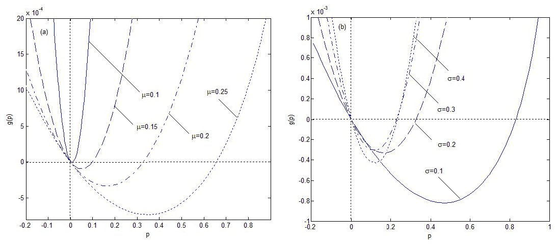
Figure 3 Curve variation in the moment Lyapunov exponent with the increase in noise parameters μ and σfor the following case: $k=\text{Cn}=\mathrm{0.4}$, d₁=0.1, d₂=0.2, A₀=1.4, B₀=1, $b_{\mathrm{11}}=b_{\mathrm{12}}=b_{\mathrm{21}}=b_{\mathrm{22}}=\mathrm{1}$.

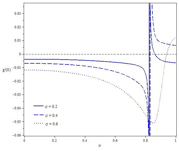
Figure 4 Variation in the maximum Lyapunov exponent with noise parameters μ and σ for the following case: $k=\text{Cn}=\mathrm{0.4}$, $d_{\mathrm{1}}=\mathrm{0.1},d_{\mathrm{2}}=\mathrm{0.2}$, A₀=1.4, B₀=1, $b_{\mathrm{11}}=b_{\mathrm{12}}=b_{\mathrm{21}}=b_{\mathrm{22}}=\mathrm{1}$.

Figure 5 Trends of the moment Lyapunov exponent with system parameters d₁ and d₂ for the following case: $k=\text{Cn}=\mathrm{0.4}$, A₀=1.4, B₀=1, $b_{\mathrm{11}}=b_{\mathrm{12}}=b_{\mathrm{21}}=b_{\mathrm{22}}=\mathrm{1}$, $\mathit{\mu }=\mathit{\sigma }=\mathrm{0.2}$.

Figure 6 Effect of system parameters k and Cn on the moment Lyapunov exponent for the following case: d₁=0.1, d₂=0.2, A₀=1.4, B₀=1, $b_{\mathrm{11}}=b_{\mathrm{12}}=b_{\mathrm{21}}=b_{\mathrm{22}}=\mathrm{1}$, $\mathit{\mu }=\mathit{\sigma }=\mathrm{0.2}$.

Figure 7 Influence of system parameters A₀ and B₀ on the moment Lyapunov exponent for the following case: $k=\text{Cn}=\mathrm{0.4}$, d₁=0.1, d₂=0.2, $b_{\mathrm{11}}=b_{\mathrm{12}}=b_{\mathrm{21}}=b_{\mathrm{22}}=\mathrm{1}$, $\mathit{\mu }=\mathit{\sigma }=\mathrm{0.2}$.

In Fig. 2, the curves of the moment Lyapunov exponent g(p) with the increased values of n for two different cases are given. The two pictures display that the deviation of the curves of the moment Lyapunov exponent is very large at n=1 and n=2, where n represents the order of the sub-matrix. However, as n=2 and n=3, the curves of g(p) are nearly coincident. Thus, we conclude that the series of the moment Lyapunov exponent are convergent when the order n of matrix R rises, and it is sufficient for us to truncate the fourth-order approximate of g₂(p).

It can be seen from the analytical expressions of the elements in matrix R that the moment Lyapunov exponents are impacted by the noise excitation. In Fig. 3, the curves of the moment Lyapunov exponent with respect to the noise parameters are described. The effects of the drift coefficient μ and diffusion coefficient σ on the moment stability are contrary. The moment stability of the system is weakened with the increase in μ, while it is enhanced with the increased σ. Furthermore, there is a bigger sensitivity near σ=0.1 because the distance of the curves between σ=0.1 and σ=0.2 is larger than among σ=0.2, 0.3 or 0.4. At the same time, the almost sure stability of the system excited by noise is also presented in Fig. 4. When σ=0.2 and 0.4, μ<0.82 and σ=0.6 and μ<0.91, the system is almost surely asymptotically stable. However, jumping between μ=0.82 and μ=0.84, the curves rapidly increase and the system becomes instable, and the trend slightly slows down a little at σ=0.6.

In addition, moment Lyapunov exponents are not only related to noise disturbance but are also affected by system parameters. The effects of the different values of damping coefficients on the moment Lyapunov exponent are shown in Fig. 5. It is obvious that the moment stability of the system is enhanced with the increase in d₁ and d₂, but the influence of d₁ on the system is stronger than that of d₂ because the variational intensity of its curves is larger. Figure 6 depicts the moment Lyapunov exponent with the increased k and Cn. The increase in k weakens the system stability, and the larger k is, the smaller the influence becomes from Fig. 6a. In Fig. 6b, all the four curves coincide completely, which indicates that different values of Cn have no effect on the system. Finally, the trends of the curves in Fig. 7a and b are just the opposite of each other, and the moment stability of the system strengthens with the increase in A₀.

6 Conclusions

In this paper, the stochastic stability of a gyro-pendulum system parametrically excited by a bounded noise is investigated through the moment Lyapunov exponent. An eigenvalue problem of the moment Lyapunov exponent is constructed by applying the theory of the stochastic dynamical system. Then, a perturbation method and Fourier cosine series expansion are used to obtain the infinite-order matrix whose leading eigenvalue is just the second-order expansion of the moment Lyapunov exponent. Furthermore, the convergence of the infinite eigenvalue sequence is numerically verified by two typical cases. Finally, the effects of system and noise parameters on the moment Lyapunov exponent are discussed. The impacts of two noise parameters on moment stability are the opposite of each other: the increase in μ makes the stability enhance, and σ has the opposite effect. Among the system parameters, only Cn has no effect on the stability, and moment stability is strengthened with the increased k and A₀, while the other parameters weaken it.