Application of cell mapping to control optimization for an antenna servo system on a disturbed carrier

The cell-mapping method, due to its global optimality, has been applied to solve multi-objective optimization problems (MOPs) and optimal control problems. However, the curse of dimensionality limits its application in high-dimensional systems. In this paper, the multi-parameter sensitivity analysis is investigated to reduce the parameter space dimension, which broadens the application of cell mapping to MOPs in high-dimensional parameter space. A post-processing algorithm for MOPs is introduced to help choose proper control parameters from the Pareto set. The proposed scheme is applied successfully in the control parameter optimization of an adaptive nonsingular terminal sliding-mode control for an antenna servo system on a disturbed carrier. Moreover, as the existing global optimal tracking control with an adjoining cell-mapping method may generate tracking-phase differences, an optimal-sliding-mode combined-control strategy is proposed. By using the combined-control strategy, the azimuth and pitch angles of the antenna system are controlled to catch up to a target trajectory with the minimum cost function and to keep high-precision tracking after that.

1 Introduction

Cell mapping is a highly efficient numerical method for the global dynamical characteristic analysis of nonlinear dynamical systems. With the cell-mapping method, a state space region is discretized into a set of cells, and the dynamical behaviors described by an infinite number of point-to-point mappings can be represented by a finite number of cell-to-cell mappings. Then, long-term global dynamical characteristics, including attractors, domains of attraction, equilibrium states, etc., can be obtained by studying short-term cell-mapping relationships. The simple cell mapping (SCM) was first proposed by Hsu (1980). After that, the cell-mapping method was developed by a lot of scholars (Dellnitz and Hohmann, 1997; Sun and Luo, 2012). Due to its powerful global analysis ability, cell mapping has been extended to control optimization fields including multi-objective optimization problems (MOPs) (Fernández et al., 2016) and optimal controls (Martínez-Marín and Zufiria, 1999).

One application of the cell-mapping method in control optimization fields is the solving of MOPs. In a control process, multiple performance indexes are usually considered to evaluate the control performance, such as overshoot, peak time, or steady-state error. The design of control parameters to meet multiple conflicting performance objective functions simultaneously as far as possible yields the multi-objective optimization problem. The traditional single-objective optimization problem has only one unique solution. But the MOP has a set of solutions, which is called the Pareto set. The corresponding optimization objective function values are named the Pareto front. Many numerical algorithms for solving MOPs have been developed, such as the immune algorithm (Chen et al., 2019), particle swarm optimization (Peng et al., 2019; Zhang et al., 2022) and the genetic algorithm (Du et al., 2016). These algorithms are mainly based on bionics. Recently, the cell-mapping method was developed as an effective numerical method to solve MOPs. The cell-mapping method to deal with MOPs is one kind of set-oriented method with subdivision technology. It is global in nature and allows one to approximate the entire set of global Pareto points. Compared with other optimization methods, it can guarantee global optimality well to a great extent and can obtain the Pareto set with one single run of the algorithm. Besides, it is applicable to a wide range of optimization problems and is characterized by an excellent robustness. The SCM was firstly used for multi-objective optimal proportion integration differentiation (PID) control for a nonlinear system with a time delay (Xiong et al., 2013). Then a hybrid algorithm consisting of gradient-based and gradient-free laws for MOPs was presented (Xiong et al., 2014), and a hybrid method consisting of the genetic algorithm and SCM was proposed (Naranjani et al., 2014). A post-processing strategy to select control parameters from the Pareto set is shown by Qin and Sun (2017). The algorithm first sets an ideal point and then circles the ideal point with a radius to narrow the selective area of optimal solutions. As mappings from different pre-image cells to their image cells need to be constructed in the cell-mapping method, it is easy to imagine that the calculation task will grow rapidly when the dimension of an analyzed dynamical system increases. Because the construction of cell-to-cell mappings are naturally parallelizable, the graph process unit (GPU) parallel technology was introduced to the global analysis with the cell-mapping method for high-dimensional nonlinear dynamical systems (Xiong et al., 2015). The MOP design of a sliding-mode control with a parallel simple cell-mapping method was studied (Qin et al., 2017). The multi-objective optimal motion control of a twin-rotor model helicopter based on the parallel simple cell-mapping method was presented (Qin et al., 2020). The cell-mapping method is an interesting alternative to the classical mathematical programming method. It has been applied successfully to lowly and moderately dimensional MOPs. However, the curse of dimensionality still exists even though the GPU parallel technology is adopted. That is the main limitation of the cell-mapping method in its application to MOPs for more control parameters.

Another application of the cell-mapping method in control optimization fields is the solving of optimal control problems. Optimal controls have been widely applied in many engineering fields (Lu et al., 2019). However, the analytic optimal control solutions are usually difficult to find for complex nonlinear systems, especially when the state space region and control inputs are constrained. The cell-mapping method provides an efficient numerical way to solve optimal control problems for complex nonlinear dynamical systems. More importantly, the cell-mapping method searches optimal control solutions in the whole state space region, which can guarantee the global optimality better compared with other methods. The SCM was firstly introduced to solve optimal control problems by Hsu (1985). The solving of fixed-final-state (Crespo and Sun, 2000) and fixed-final-time (Crespo and Sun, 2003) optimal control problems with SCM was studied. To decrease discretization error, the adjoining cell-mapping method was investigated to solve optimal control problems by Zufiria and Martínez-Marín (2003). The optimal control with the adjoining cell mapping performs closed-loop feedback control, which makes it applicable in real physical systems. As for optimal tracking control problems, even numerical solutions are difficult to obtain. The SCM was used for optimal control of tracking moving targets with a bounded state space region by Crespo and Sun (2001), but it was limited to only low-dimension single-input–single-output systems. Recently, a subdivision strategy of adjoining cell mapping was proposed to deal with fixed-final-state global optimal control problems for multi-input–multi-output (MIMO) systems (Cheng and Jiang, 2021), and it was extended to solve the global optimal tracking control for MIMO systems (Tian et al., 2023). However, the low steady-state tracking accuracy and the existence of phase differences between the target trajectory and the real trajectory limit the application of adjoining cell mapping to a wider range of optimal control problems.

In brief, on the one hand, the cell-mapping method is still limited by enormous calculations when dealing with the MOP in high-dimensional parameter space. On the other hand, the global optimal control with the cell-mapping method is currently mainly focused on low-latitude single-input–single-output dynamical systems. Even the subdivision strategy for adjoining cell mapping has been proposed to solve fixed-final-state global optimal controls and global optimal tracking controls for MIMO systems; further research should still be conducted. Therefore, in this paper, the MOP with the cell-mapping method in high-dimensional parameter space is studied, and the global optimal tracking control with the cell-mapping method for nonlinear MIMO systems is investigated. The proposed approaches are applied in the control optimization for a MIMO antenna servo system on a disturbed carrier.

This paper is organized as follows. The modeling and adaptive nonsingular terminal-sliding mode control (ANTSMC) design for the antenna servo system are described in Sect. 2. In Sect. 3, the control parameters' multi-objective optimization for ANTSMC based on multi-parameter sensitivity analysis and simple cell mapping is illustrated, and a post-processing algorithm for MOPs is introduced. In Sect. 4, an optimal-sliding-mode combined-control (OSCC) strategy is proposed and applied in the global optimal tracking control for the antenna servo system. Finally, Sect. 5 concludes the paper. The main contributions of this paper are as follows:

• 1.

  The multi-parameter sensitivity analysis is adopted to reduce the dimension of parameter space, which broadens the application of the cell-mapping method to MOPs in high-dimensional parameter space.

• 2.

  A post-processing algorithm for MOPs is introduced, which can help to select proper control parameters from the Pareto set.

• 3.

  An optimal-sliding-mode combined-control strategy is proposed, which offers a widely applicable and efficient numerical way to solve optimal tracking control problems for nonlinear MIMO systems in engineering.

2 The system description and sliding-mode control design

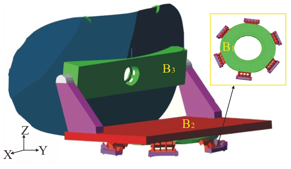
The antenna system on a mobile carrier has the advantage of real-time communication without the limitation of geographical conditions. It has already been widely applied in the fields of battlefield communications, emergency communication, rescue operations and television relay. An antenna system on a mobile carrier consists of many components, including an antenna, electrical motors, inertial navigation devices and so on. As the carrier is always under external, large disturbance, it is difficult to control the antenna attitude quickly and accurately by means of the classical PID strategy. Consequently, the dynamical modeling is necessary for the control design. The sketch map of an antenna system on a mobile carrier is shown in Fig. 1. Wire-cable vibration isolation equipment B₁ with a hysteretic-damping characteristic is adopted to isolate the disturbance from the carrier. To facilitate modeling, the whole system is simplified as a multi-rigid-body system with four rigid bodies: the vibration isolation equipment B₁, the azimuth turntable B₂, the pitch turntable B₃ and a carrier which is not depicted in Fig. 1. There are 5 generalized degrees of freedom for this system in total. The system can be described by the nonlinear multi-body dynamical equations:

$$\begin{array}{}\text{(1)}& \begin{array}{rl}& \left[\begin{array}{ccccc}{A}_{\mathit{\alpha }\mathrm{1}}& A_{\mathit{\alpha }\mathrm{2}}& A_{\mathit{\alpha }\mathrm{3}}& A_{\mathit{\alpha }\mathrm{4}}& A_{\mathit{\alpha }\mathrm{5}}\\ A_{\mathit{\beta }\mathrm{1}}& A_{\mathit{\beta }\mathrm{2}}& A_{\mathit{\beta }\mathrm{3}}& A_{\mathit{\beta }\mathrm{4}}& A_{\mathit{\beta }\mathrm{5}}\\ A_{\mathrm{11}}& A_{\mathrm{12}}& A_{\mathrm{13}}& \mathrm{0}& \mathrm{0}\\ A_{\mathrm{21}}& A_{\mathrm{22}}& \mathrm{0}& A_{\mathrm{24}}& \mathrm{0}\\ A_{\mathrm{31}}& A_{\mathrm{32}}& \mathrm{0}& \mathrm{0}& A_{\mathrm{35}}\end{array}\right]\left[\begin{array}{c}\ddot{\mathit{\alpha }}\\ \ddot{\mathit{\beta }}\\ {\ddot{q}}_{\mathrm{1}}\\ {\ddot{q}}_{\mathrm{2}}\\ {\ddot{q}}_{\mathrm{3}}\end{array}\right]\\ & =\left[\begin{array}{c}-M_{\mathrm{3}}\sin q_{\mathrm{2}}+M_{\mathit{\alpha }}\\ -M_{\mathrm{3}}\cos q_{\mathrm{2}}+M_{\mathit{\beta }}\\ F-\left(m_{\mathrm{1}}+m_{\mathrm{2}}+m_{\mathrm{3}}\right)g\\ M_{\mathrm{2}}\\ M_{\mathrm{3}}\end{array}\right]+\left[\begin{array}{c}{R}_{\mathit{\alpha }}\\ R_{\mathit{\beta }}\\ R_{\mathrm{1}}\\ R_{\mathrm{2}}\\ R_{\mathrm{3}}\end{array}\right].\end{array}\end{array}$$

In Eq. (1), α and β are the relative rotation angles of B₁ to the carrier in X and Y direction, q₁ is the relative translation displacement of B₁ to the carrier in Z direction, q₂ is the azimuth rotation angle of B₂ to B₁, and q₃ is the pitch rotation angle of B₃ to B₂. M₂(t) and M₃(t) are azimuth and pitch external-control moment inputs, respectively. M_α, M_β and F are, respectively, the moments in X and Y direction and the resultant force in Z direction acting on B₂ arising from B₁. m₁, m₂ and m₃ are the mass of B₁, B₂ and B₃. The other coefficients in Eq. (1) contain large amounts of coupling terms with the 10 variables and their trigonometric functions, as well as the angular velocity and acceleration of the carrier. So this MIMO system displays strong nonlinearity.

Figure 1 The sketch map of the antenna system.

As the sliding-mode control possesses good robustness against external disturbance, it is adopted to control the antenna attitude angles for this servo system. The control objective is to make the azimuth q₂ and pitch q₃ track a given trajectory, and the control errors are set as

$$\begin{array}{}\text{(2)}& \left\{\begin{array}{l}{e}_{\mathrm{2}}=q_{\mathrm{2}}-q_{\mathrm{20}}\\ e_{\mathrm{3}}=q_{\mathrm{3}}-q_{\mathrm{30}}\end{array}\right.,\end{array}$$

where q₂₀ and q₃₀ are control targets. The non-singular terminal-sliding mode variables are designed as

$$\begin{array}{}\text{(3)}& \left\{\begin{array}{l}{s}_{\mathrm{2}}=e_{\mathrm{2}}-{\mathit{\beta }}_{\mathrm{2}}{\left|{\dot{e}}_{\mathrm{2}}\right|}^{{\mathit{\gamma }}_{\mathrm{2}}}\text{sgn}\left({\dot{e}}_{\mathrm{2}}\right)\\ s_{\mathrm{3}}=e_{\mathrm{3}}-{\mathit{\beta }}_{\mathrm{3}}{\left|{\dot{e}}_{\mathrm{3}}\right|}^{{\mathit{\gamma }}_{\mathrm{3}}}\text{sgn}\left({\dot{e}}_{\mathrm{3}}\right)\end{array}\right.,\end{array}$$

where β₂>0, β₃>0, ${\mathit{\gamma }}_{\mathrm{2}}=p_{\mathrm{21}}/p_{\mathrm{22}}$, and ${\mathit{\gamma }}_{\mathrm{3}}=p_{\mathrm{31}}/p_{\mathrm{32}}$ (p₂₁, p₂₂, p₃₁ and p₃₂ are positive odd integers, $\mathrm{1}<p_{\mathrm{21}}/p_{\mathrm{22}}<\mathrm{2}$, and $\mathrm{1}<p_{\mathrm{31}}/p_{\mathrm{32}}<\mathrm{2}$). To shorten reaching time and to weaken chattering, an adaptive variable-speed exponential-reaching law (Cheng and Jiang, 2019) is adopted

$$\begin{array}{}\text{(4)}& \dot{s}=-\mathit{\epsilon }{\displaystyle \frac{\mathrm{1}}{\mathrm{1}+c_{\mathrm{1}}\left|e\right|}}\text{sgn}\left(s\right)-\left(k+c_{\mathrm{2}}\left|e\right|\right)s,\end{array}$$

where k>0, ε>0, c₁>0, and c₂>0. The adaptive variable-speed exponential-reaching law has two parts: $-\left(k+c_{\mathrm{2}}\left|e\right|\right)$ is the exponential-reaching item, which can adjust the reaching speed according to the value of e. c₂ should be assigned a relatively large value to shorten the reaching time. $-\mathit{\epsilon }\frac{\mathrm{1}}{\mathrm{1}+c_{\mathrm{1}}\left|e_{\mathrm{1}}\right|}$ is the constant-reaching item. It is less than ε if the coefficient c₁ is assigned a relatively large value, which can weaken the chattering effectively. However, a too-large value of c₁ will result in a small value of the constant-reaching item, which may lead to the increase of the reaching time again. Therefore, c₁ should be assigned a relatively small value, while c₂ should be assigned a relatively large value. The control inputs M₂ and M₃ can be derived by the adaptive nonsingular terminal-sliding mode control (ANTSMC) as follows:

$$\begin{array}{}\text{(5)}& \left\{\begin{array}{l}\begin{array}{rl}{M}_{\mathrm{2}}& =-R_{\mathrm{2}}-A_{\mathrm{24}}\left({\displaystyle \frac{{\mathit{\epsilon }}_{\mathrm{2}}}{\mathrm{1}+c_{\mathrm{21}}\left|e_{\mathrm{2}}\right|}}\text{sgn}\right(s_{\mathrm{2}})\\ & +\left(k_{\mathrm{2}}+c_{\mathrm{22}}\left|e_{\mathrm{2}}\right|\right)s_{\mathrm{2}}-{\ddot{q}}_{\mathrm{20}}+{\displaystyle \frac{\mathrm{1}}{{\mathit{\beta }}_{\mathrm{2}}{\mathit{\gamma }}_{\mathrm{2}}}}{\left|{\dot{e}}_{\mathrm{2}}\right|}^{\mathrm{2}-{\mathit{\gamma }}_{\mathrm{2}}})\end{array}\\ \begin{array}{rl}{M}_{\mathrm{3}}& =-R_{\mathrm{3}}-A_{\mathrm{35}}\left({\displaystyle \frac{{\mathit{\epsilon }}_{\mathrm{3}}}{\mathrm{1}+c_{\mathrm{31}}\left|e_{\mathrm{3}}\right|}}\text{sgn}\right(s_{\mathrm{3}})\\ & +\left(k_{\mathrm{3}}+c_{\mathrm{32}}\left|e_{\mathrm{3}}\right|\right)s_{\mathrm{3}}-{\ddot{q}}_{\mathrm{30}}+{\displaystyle \frac{\mathrm{1}}{{\mathit{\beta }}_{\mathrm{3}}{\mathit{\gamma }}_{\mathrm{3}}}}{\left|{\dot{e}}_{\mathrm{3}}\right|}^{\mathrm{2}-{\mathit{\gamma }}_{\mathrm{3}}})\end{array}\end{array}\right.,\end{array}$$

where β₂>0, β₃>0, $\mathrm{1}<{\mathit{\gamma }}_{\mathrm{2}}<\mathrm{2}$, $\mathrm{1}<{\mathit{\gamma }}_{\mathrm{3}}<\mathrm{2}$, k₂>0, k₃>0, ε₂>0, ε₃>0, c₂₁>0, c₂₂>0, ε₃₁>0, and ε₃₂>0.

3 Multi-objective optimization based on sensitivity analysis and cell mapping

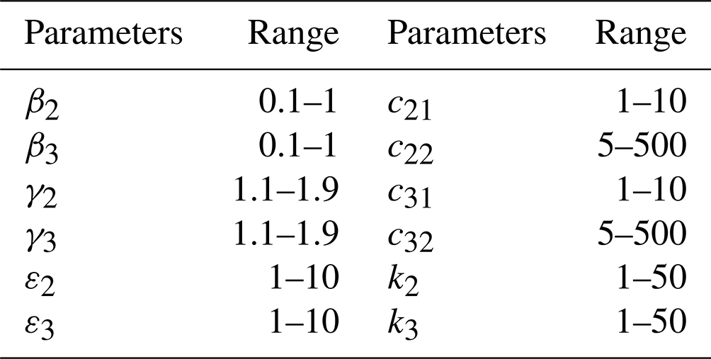
To improve the control performance of ANTSMC, control parameter optimization is necessary. The designed control parameter vector is $\mathit{k}=\left[{\mathit{\epsilon }}_{\mathrm{2}},{\mathit{\epsilon }}_{\mathrm{3}},{\mathit{\beta }}_{\mathrm{2}},{\mathit{\beta }}_{\mathrm{3}},{\mathit{\gamma }}_{\mathrm{2}},{\mathit{\gamma }}_{\mathrm{3}},k_{\mathrm{2}},k_{\mathrm{3}},c_{\mathrm{21}},c_{\mathrm{31}},c_{\mathrm{22}},c_{\mathrm{32}}\right]$, and the value ranges of these parameters are shown in Table 1. As can be seen from the table, there are multiple control parameters within wide value ranges which have an influence over the control performance. For example, the steady-state error is usually affected by the sliding-mode surface parameters β₂, β₃, γ₂ and γ₃. The overshoot and peak time are affected by the reaching-law parameters γ₂, γ₃, k₂, k₃, c₂₁, c₃₁, c₂₂ and c₃₂, and they are always conflicting. As the controlled system is strongly nonlinear, how to adjust the 12 control parameters to meet multiple objective functions simultaneously as far as possible is a thorny problem. The design of the control parameters to meet multiple conflicting objectives in an optimal manner leads to a multi-objective optimization problem (MOP).

Table 1 The value ranges of ANTSMC parameters.

The overshoot, peak time and steady-state error are usually used to characterize the performance of the closed-loop feedback control. The MOP in this paper can be described as

$$\begin{array}{}\text{(6)}& \underset{\mathit{k}\in \mathrm{\Omega }}{min}\mathbf{F}=\underset{\mathit{k}\in \mathrm{\Omega }}{min}\left\{O_{q_{\mathrm{2}}},O_{q_{\mathrm{3}}},T_{{\mathrm{p}}_{q_{\mathrm{2}}}},T_{{\mathrm{p}}_{q_{\mathrm{3}}}},E_{q_{\mathrm{2}}},E_{q_{\mathrm{3}}}\right\},\end{array}$$

where Ω is the set of the control parameter vector k, $O_{q_i}$ is the overshoot of q_i, $T_{{\mathrm{p}}_{q_i}}$ is the peak time of q_i, and $E_{q_i}$ evaluates the steady-tracking error of q_i and has the form

$$\begin{array}{}\text{(7)}& E_{q_i}={\int }_{T_{\mathrm{s}}}^{T_{\mathrm{e}}}{\left(q_i\left(t\right)-q_{i\mathrm{0}}\right)}^{\mathrm{2}}\mathrm{d}t,\end{array}$$

where T_s is a certain moment when the tracking control is in the steady state, and T_e is the end time. In order to ensure good control performance, the objective functions are constrained by

$$\begin{array}{}\text{(8)}& \begin{array}{rl}[& O_{q_{\mathrm{2}}}<\mathrm{1}\mathit{\%},O_{q_{\mathrm{3}}}<\mathrm{1}\mathit{\%},T_{{\mathrm{p}}_{q_{\mathrm{2}}}}<\mathrm{3}\mathrm{s},T_{{\mathrm{p}}_{q_{\mathrm{3}}}}<\mathrm{3}\mathrm{s},\\ & E_{q_{\mathrm{2}}}<{\mathrm{10}}^{-\mathrm{6}},E_{q_{\mathrm{3}}}<{\mathrm{10}}^{-\mathrm{6}}].\end{array}\end{array}$$

In the simulation in this paper, the end time is set as T_e=5 s, and T_s is set as T_s=4 s to ensure that the tracking control has been in the steady state. The carrier is assumed under the disturbance that its angular velocities in X, Y and Z direction move sinusoidally with an amplitude of 10^∘ and a period of 2 s.

The cell-mapping method to deal with MOPs can find the global and fine structure of the Pareto set through one single run of the program. Although the global optimality can be guaranteed well, the computational time required increases dramatically when the dimension of the design parameter space increases. Consequently, it is poorly suited to dealing with MOPs in high-dimension parameter space due to the curse of dimensionality. In this paper, we consider the use of sensitivity analysis technology to realize the dimensionality reduction of the parameter space effectively.

3.1 Sensitivity analysis

There are 12 control parameters in the ANTSMC design for the antenna system. Direct optimization of the 12 control parameters will consume too much computation, which is not cost-effective and is even unfeasible. In fact, these parameters may have different influences on the change of the objective function values. When these parameters change simultaneously, some may play relatively important roles in the system output response compared with the others. Consequently, it is easy to imagine that the relatively important control parameters can be optimized first and the others after that. In this way, the dimensionality of the parameter space is reduced, which greatly economizes the computational cost, and the approximate MOP solutions can be obtained with sufficient accuracy.

This brings us to the next problem of how to assess the influence of each control parameter on the objective functions of the decision maker. The main purpose of parameter sensitivity analysis is to evaluate the importance of each input parameter to the system output. There are two main methods for sensitivity analysis: single-parameter sensitivity analysis and multi-parameter sensitivity analysis. Among them, the multi-parameter sensitivity analysis method allows the situation in which multiple parameters change simultaneously, which has global significance. The Sobol method (Sobol and Kucherenko, 2009) is a classical and sophisticated and the most widely used multi-parameter sensitivity analysis method. It is a sort of Monte Carlo method based on variance and has the advantages of fast convergence and good stability. It also has good applicability in the situation of obvious multiple-parameter interactions in the strongly nonlinear systems. Moreover, the first-order, second-order and high-order global sensitivity coefficients can be obtained simultaneously. The Sobol method divides the total variance into the independent variance and the interaction variance between different parameters. A function $Y=f(X_{\mathrm{1}}{X}_{\mathrm{2}},\mathrm{\dots },X_n)$ can be divided into a set of functions with increased dimensions, and the first-order sensitivity coefficient of a parameter X_i can be expressed as

$$\begin{array}{}\text{(9)}& S_i={\displaystyle \frac{V\left[E\left(Y\mathrm{|}{X}_i\right)\right]}{V\left[Y\right]}},\end{array}$$

where E(Y | X_i) is the conditional expectation, and V is the variance. The total sensitivity coefficient of X_i is denoted as

$$\begin{array}{}\text{(10)}& S_{T_i}={\displaystyle \frac{E\left[V\left(Y\mathrm{|}{X}_{\sim i}\right)\right]}{V\left[Y\right]}}=\mathrm{1}-{\displaystyle \frac{V\left[E\left(Y\mathrm{|}{X}_{\sim i}\right)\right]}{V\left[Y\right]}}\end{array}$$

where X_∼i is all the parameters in X except X_i.

To avoid a sampling-centralization phenomenon, Latin hypercube sampling (LHS) is adopted, which can better cover the parameter space region with a small number of samples. LHS is widely used in the probability statistics of complex systems with random input characteristics. In multi-parameter sensitivity analysis, LHS is an important and commonly used parameter sample acquisition method. The main idea of LHS is to make uniform equal-probability stratification for each dimension of the parameter space and then to select samples from each layer randomly. In order to improve computation speed, two-time independent samples (Saltelli, 2002) are executed. The generated vector samples are scrambled and rearranged subsequently.

To execute parameter sensitivity analysis of ANTSMC for the antenna servo system, 10 000 groups of control parameters are sampled, and two independent samples are taken. In Fig. 2, the sensitivity coefficient of β₂ for the objective function $O_{q_{\mathrm{2}}}$ is presented. When the number of samples is over about 2000, the sensitivity coefficient of ε₂ holds steady at approximately 0.15. The sensitivity coefficients of other control parameters for different objective functions follow the similar regular pattern. The sensitivity analysis result of each control parameter for different objective functions is shown in Table 2. It can be seen from the table that, among all the control parameters, β₂, ε₂ and c₂₂ have a relatively large influence on $O_{q_{\mathrm{2}}}$, while β₂, β₃, ε₂, ε₃ and c₃₂ have a relatively large influence on $O_{q_{\mathrm{3}}}$. The control parameters related to q₂ also have an influence on $O_{q_{\mathrm{3}}}$, which is due to the existence of couplings. β₂, γ₂ and c₂₂ have a greater impact on peak time $T_{{\mathrm{p}}_{q_{\mathrm{2}}}}$, while β₃, γ₃ and c₃₂ have a greater impact on $T_{{\mathrm{p}}_{q_{\mathrm{3}}}}$. $E_{q_{\mathrm{2}}}$ is mainly affected by β₂ and γ₂, while $E_{q_{\mathrm{3}}}$ is mainly affected by β₃ and γ₃, which is consistent with the fact that the steady-state performance of the sliding-mode control only depends on the parameters of the sliding-mode surface.

Figure 2 Sensitivity coefficient convergence curve of β₂ for $O_{q_{\mathrm{2}}}$.

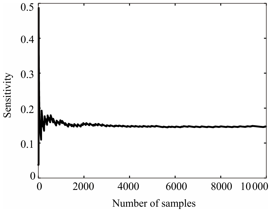
Table 2 Parameter sensitivity analysis results and importance evaluation. The sensitivity coefficients playing important roles are highlighted in bold.

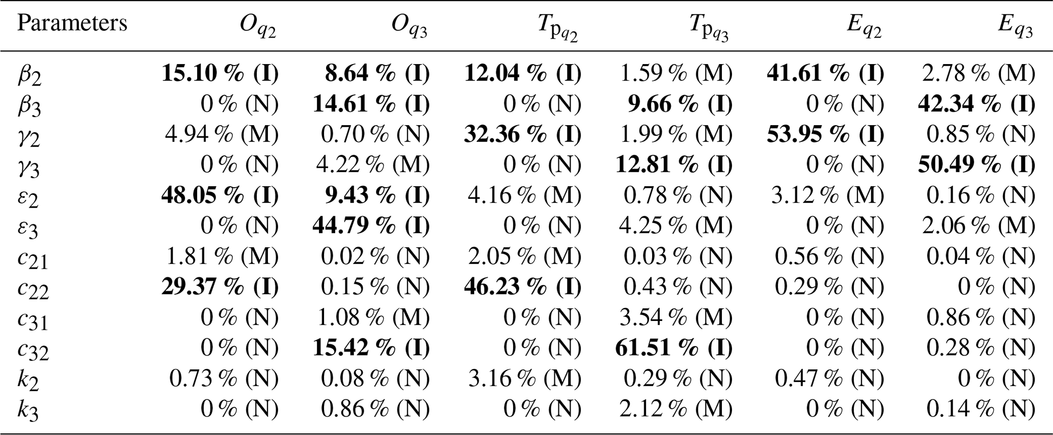
To make the sensitivity analysis results more visible, it is assumed that, if the sensitivity coefficient of a parameter for an objective function is greater than 5 %, the parameter is considered to be important to this objective function; if the sensitivity coefficient is less than 1 %, the parameter is considered to negligible in relation to this objective function; if the sensitivity coefficient is between 1 % and 5 %, the parameter is relatively minorly important to this objective function. According to multi-parameter sensitivity results, the importance of each parameter to different objective functions is evaluated and also shown in Table 2. The symbols I, M and N indicate important, minorly important and negligible, respectively. Table 2 shows that there are four parameters which have no important impact on all objective functions, namely k₂, k₃, c₂₁ and c₃₁. In fact, the maximal one among the sensitivity coefficients of the four control parameters for one objective function is merely 3.16 %. This means that the 4 control parameters have quite a small influence on all the objective functions compared with the other 8 parameters when the 12 parameters change simultaneously. Consequently, it can be easily deduced that the MOP described by Eq. (6) can be simplified approximately as the optimization of eight relatively important parameters firstly and the other four parameters next. In this way, the dimension of the parameter space decreases from 12 to 8, which makes the MOP with the cell-mapping method achievable.

3.2 Multi-objective optimization with simple cell mapping

The cell-mapping method to solve MOPs can obtain the Pareto optimal set through one single run of the algorithm and can ensure the global optimization well. With the cell-mapping method, a region in the parameter space is discretized into uniform cells. An infinite number of points in the parameter space can be represented by a finite number of cells. In simple cell mapping (SCM), the characteristics of a cell are represented by the characteristics of its center point. The Pareto optimal set is obtained by constructing cell-to-cell mappings in the parameter space and extracting the periodic cells.

The objective function value corresponding to the center point of each cell is calculated firstly, and the free gradient law (Qin et al., 2017) is adopted to construct one-step simple cell mapping. Let ${\mathbf{z}}_{k_n}$ represent the cell corresponding to its center point parameter vector k_n. The free gradient law determines the image cell of a cell ${\mathbf{z}}_{k_n}$ by comparing the objective function values of the cell with those its neighborhood cells. If there exists a neighborhood cell ${\mathbf{z}}_{k_i}$ whose objective function value satisfies the conditions F(k_i)≤F(k_n) and F(k_i)≠F(k_n), ${\mathbf{z}}_{k_i}$ is regarded as the image cell of the pre-image cell ${\mathbf{z}}_{k_n}$. If there exists more than one neighborhood whose objective function values satisfy the aforementioned condition, the maximally dominant cell in the neighborhood is treated as the image cell. The mapping relationship can be expressed as

$$\begin{array}{}\text{(11)}& {\mathbf{z}}_{k_n}=C^{\mathrm{s}}\left({\mathbf{z}}_{k_i}\right).\end{array}$$

If there exists no image cell of ${\mathbf{z}}_{k_n}$, ${\mathbf{z}}_{k_n}$ is recognized as a periodic cell under the concept of MOP with SCM, and the corresponding control parameter group is considered to be a Pareto optimal candidate. All the information of the Pareto optimal set is contained in the one-step cell mappings. After all the periodic cells are found, the dominance relationship checking is instituted to avoid the local Pareto optimal solutions, which can ensure the global optimality. Each periodic cell is compared with other periodic cells, and only those periodic cells which are not dominated by any other periodic cell constitute the Pareto optimal set.

To improve calculation speed, the subdivision technology and GPU parallel technology are adopted. Recall the MOP described in Eq. (6). The parameter space region is firstly discretized as 5⁸ relatively coarse cells. The objective function values corresponding to every center point vector of these cells are firstly calculated by GPU parallel technology, and the constraint condition described by Eq. (8) is checked. If the constraint condition is satisfied, the corresponding cell is considered to be processed next to find its image cell. If the constraint condition is not satisfied, the corresponding cell is discarded. After the mapping relationship judgment, 153 coarse periodic cells are found whose center vectors represent the Pareto optimal set candidates.

Then each coarse periodic cell is further discretized as 5⁸ smaller cells. Consequently, the final partition scale of the parameter space region is 25⁸. The calculation of objective function values, the constraint condition judgment and the search for periodic cells are executed again. The final Pareto optimal set contains 1012 fine cells after the dominance relationship checking. Figure 3a and b show the projections of the Pareto set on 3D sub-spaces (β₂, γ₂, ε₂) and (ε₃, β₃, c₃₂). The projections of the Pareto front on 2D planes ($T_{{\mathrm{p}}_{q_{\mathrm{2}}}}$, $E_{q_{\mathrm{2}}}$) and ($O_{q_{\mathrm{3}}}$, $T_{{\mathrm{p}}_{q_{\mathrm{3}}}}$) are exhibited in Fig. 3c and d, respectively. The Pareto front displays the contradictory relationship between different objective functions well. The parallel calculation is instituted on a GPU device (NVIDIA GeForce GTX 1080Ti graphics card), which has 3584 cores with a frequency of 1480 MHz.

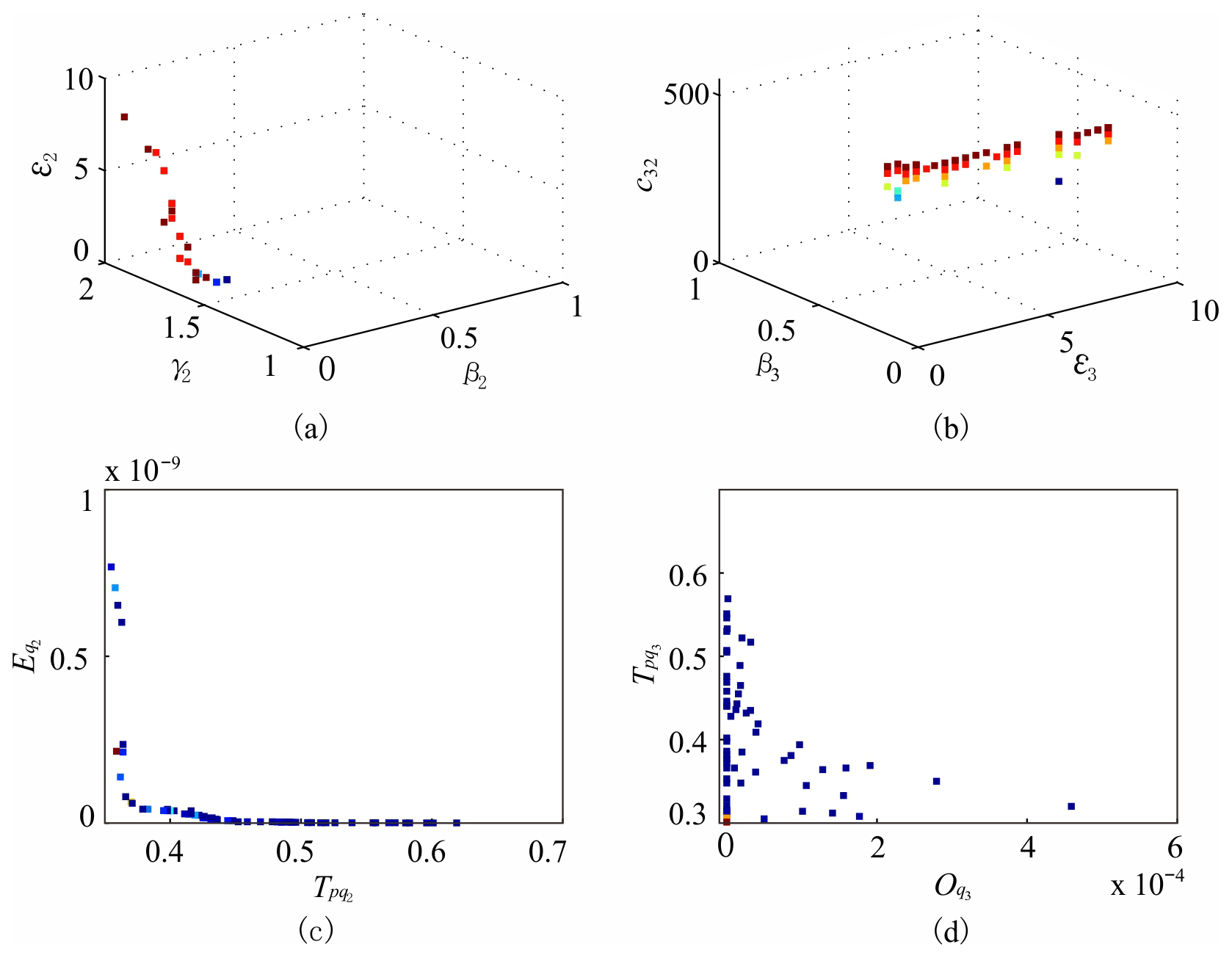
Figure 3 The projections of the Pareto set on 3D sub-spaces (a) (β₂, γ₂, ε₂) and (b) (ε₃, β₃, c₃₂) and the projections of the Pareto front on 2D planes (c) ($T_{{\mathrm{p}}_{q_{\mathrm{2}}}}$, $E_{q_{\mathrm{2}}}$) and (d) ($O_{q_{\mathrm{3}}}$, $T_{{\mathrm{p}}_{q_{\mathrm{3}}}}$). The color code indicates the level of (a) c₂₂, (b) γ₃, (c) $O_{q_{\mathrm{2}}}$ and (d) $E_{q_{\mathrm{3}}}$: red in the color code indicates the highest level, while dark blue indicates the lowest level.

3.3 Post-processing algorithm

A set of points in the parameter space which represent the Pareto optimal solutions is obtained after the MOP solving. Usually, the multi-objective optimal control design generates hundreds or thousands of Pareto optimal solutions. How the decision maker selects appropriate control parameters from the Pareto set is a post-processing issue. In this paper, a post-processing algorithm for MOPs is introduced. For every objective function F_i, the difference between the maximum value $F_i^{max}$ and the minimum value $F_i^{min}$ is recognized first. Then it is divided equally by a fixed positive integer N:

$$\begin{array}{}\text{(12)}& h_i=(F_i^{max}-F_i^{min})/N,i=\mathrm{1},\mathrm{2},\mathrm{\dots },n_{\mathrm{F}},\end{array}$$

where n_F is the total number of the objective function. Subsequently, the weight coefficient η_i is designed for every objective function according to the willingness of the decision maker, and a distance r_i is set as

$$\begin{array}{}\text{(13)}& r_i^j=F_i^{min}+j{\mathit{\eta }}_i{h}_i,i=\mathrm{1},\mathrm{2},\mathrm{\dots },n_F,j=\mathrm{1},\mathrm{2},\mathrm{\dots },N.\end{array}$$

The region $\left[F_i^{min},r_i^j\right]$ is used to pick the Pareto front and the corresponding Pareto optimal solutions.

With the post-processing algorithm, the Pareto front obtained by solving the MOP of the ANTSMC parameters is processed. N is assigned as 100, and η_i as $(\mathrm{0.8},\mathrm{0.8},\mathrm{0.4},\mathrm{0.4},\mathrm{0.3},\mathrm{0.3})$, which corresponds to $(O_{q_{\mathrm{2}}},O_{q_{\mathrm{3}}},T_{{\mathrm{p}}_{q_{\mathrm{2}}}},T_{{\mathrm{p}}_{q_{\mathrm{3}}}},E_{q_{\mathrm{2}}},E_{q_{\mathrm{3}}}$). After the post-processing algorithm, the top 22 % of the Pareto optimal solutions are picked up from the original 1012 ones. Figure 4a and b show the projections of the Pareto set on 3D sub-spaces (β₂, γ₂, ε₂) and (ε₃, β₃, c₃₂) after post-processing, while Fig. 4c and d show the projections of the Pareto front on 2D planes ($T_{{\mathrm{p}}_{q_{\mathrm{2}}}}$, $E_{q_{\mathrm{2}}}$) and ($O_{q_{\mathrm{3}}}$, $T_{{\mathrm{p}}_{q_{\mathrm{3}}}}$) after post-processing. The objective functions fall in the following range:

$$\begin{array}{}\text{(14)}& \begin{array}{rl}& \mathrm{0}\le O_{q_{\mathrm{2}}}\le \mathrm{0.0014}\mathit{\%},\mathrm{0}\le O_{q_{\mathrm{3}}}\le \mathrm{0.021}\mathit{\%},\\ & \mathrm{0.376}\le T_{{\mathrm{p}}_{q_{\mathrm{2}}}}\le \mathrm{0.416},\mathrm{0.305}\le T_{{\mathrm{p}}_{q_{\mathrm{3}}}}\le \mathrm{0.369},\\ & \mathrm{3.682}\times {\mathrm{10}}^{-\mathrm{11}}\le E_{q_{\mathrm{2}}}\le \mathrm{1.684}\times {\mathrm{10}}^{-\mathrm{10}},\\ & \mathrm{0.796}\times {\mathrm{10}}^{-\mathrm{9}}\le E_{q_{\mathrm{3}}}\le \mathrm{1.672}\times {\mathrm{10}}^{-\mathrm{9}}.\end{array}\end{array}$$

These remaining control parameter groups after the post-processing algorithm possess relatively balanced and close performance under the setting of the weight coefficient η_i. We choose one group from them arbitrarily to carry out the time domain simulation, namely ${\mathit{\beta }}_{\mathrm{2}}={\mathit{\beta }}_{\mathrm{3}}=\mathrm{0.06}$, γ₂=1.62, γ₃=1.66, ε₂=3.4, ε₃=6.2, c₂₂=490 and c₃₂=470. The other four control parameters are optimized with the same manner and are set as $c_{\mathrm{21}}={\mathit{\epsilon }}_{\mathrm{32}}=\mathrm{5}$, k₂=36 and k₃=16. To verify the effectiveness of parameter optimization, the feedback control is instituted with two different groups of control parameters. They are the optimized parameters above and the original unoptimized parameters which are adjusted artificially (Cheng and Jiang, 2019): $k_{\mathrm{2}}=k_{\mathrm{3}}={\mathit{\epsilon }}_{\mathrm{3}}=\mathrm{5}$, ε₂=2, ${\mathit{\beta }}_{\mathrm{2}}={\mathit{\beta }}_{\mathrm{3}}=\mathrm{0.5}$, ${\mathit{\gamma }}_{\mathrm{2}}={\mathit{\gamma }}_{\mathrm{3}}=\mathrm{1.5}$, $c_{\mathrm{21}}=c_{\mathrm{31}}=\mathrm{5}$ and $c_{\mathrm{22}}=c_{\mathrm{32}}=\mathrm{500}$. Figure 5 shows the time history curves and the steady-state error curves of q₂ and q₃ under the two groups of control parameters. By using the optimized parameters, the peak time $T_{{\mathrm{p}}_{q_{\mathrm{2}}}}$ decreases from 1.497 to 0.386 s, while $T_{{\mathrm{p}}_{q_{\mathrm{3}}}}$ decreases from 1.377 to 0.343 s. The steady-state error index $E_{q_{\mathrm{2}}}$ decreases from $\mathrm{3.282}\times {\mathrm{10}}^{-\mathrm{9}}$ to $\mathrm{5.721}\times {\mathrm{10}}^{-\mathrm{11}}$, while $E_{q_{\mathrm{3}}}$ decreases from $\mathrm{3.913}\times {\mathrm{10}}^{-\mathrm{8}}$ to $\mathrm{9.415}\times {\mathrm{10}}^{-\mathrm{10}}$. The control performance was improved significantly by the optimization design.

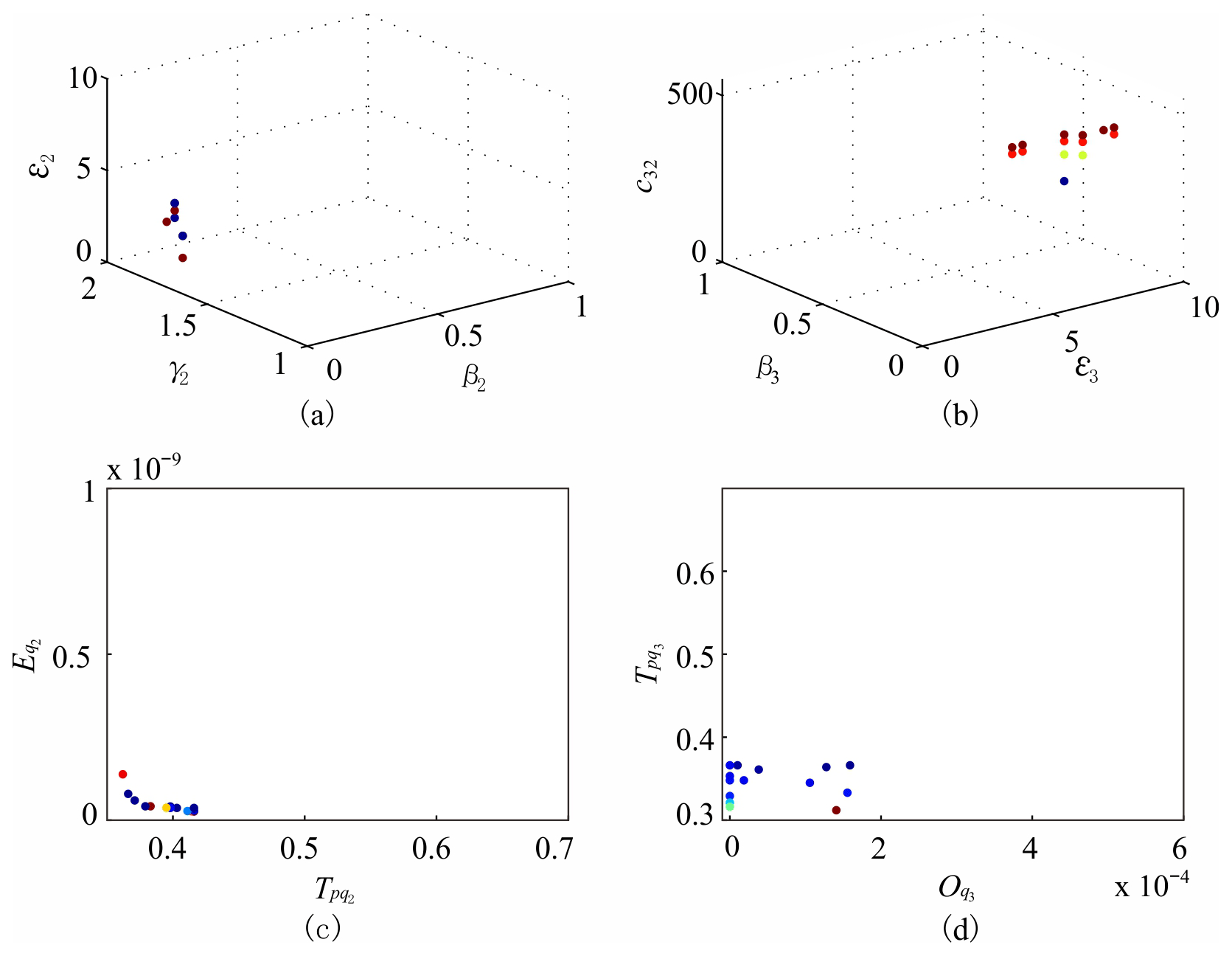
Figure 4 The projections of the Pareto set on 3D sub-spaces (a) (β₂, γ₂, ε₂) and (b) (ε₃, β₃, c₃₂) and the projections of the Pareto front on 2D planes (c) ($T_{{\mathrm{p}}_{q_{\mathrm{2}}}}$, $E_{q_{\mathrm{2}}}$) and (d) ($O_{q_{\mathrm{3}}}$, $T_{{\mathrm{p}}_{q_{\mathrm{3}}}}$) after post-processing. The color code indicates the level of (a) c₂₂, (b) γ₃, (c) $O_{q_{\mathrm{2}}}$ and (d) $E_{q_{\mathrm{3}}}$. Red in the color code indicates the highest level, while dark blue indicates the lowest level.

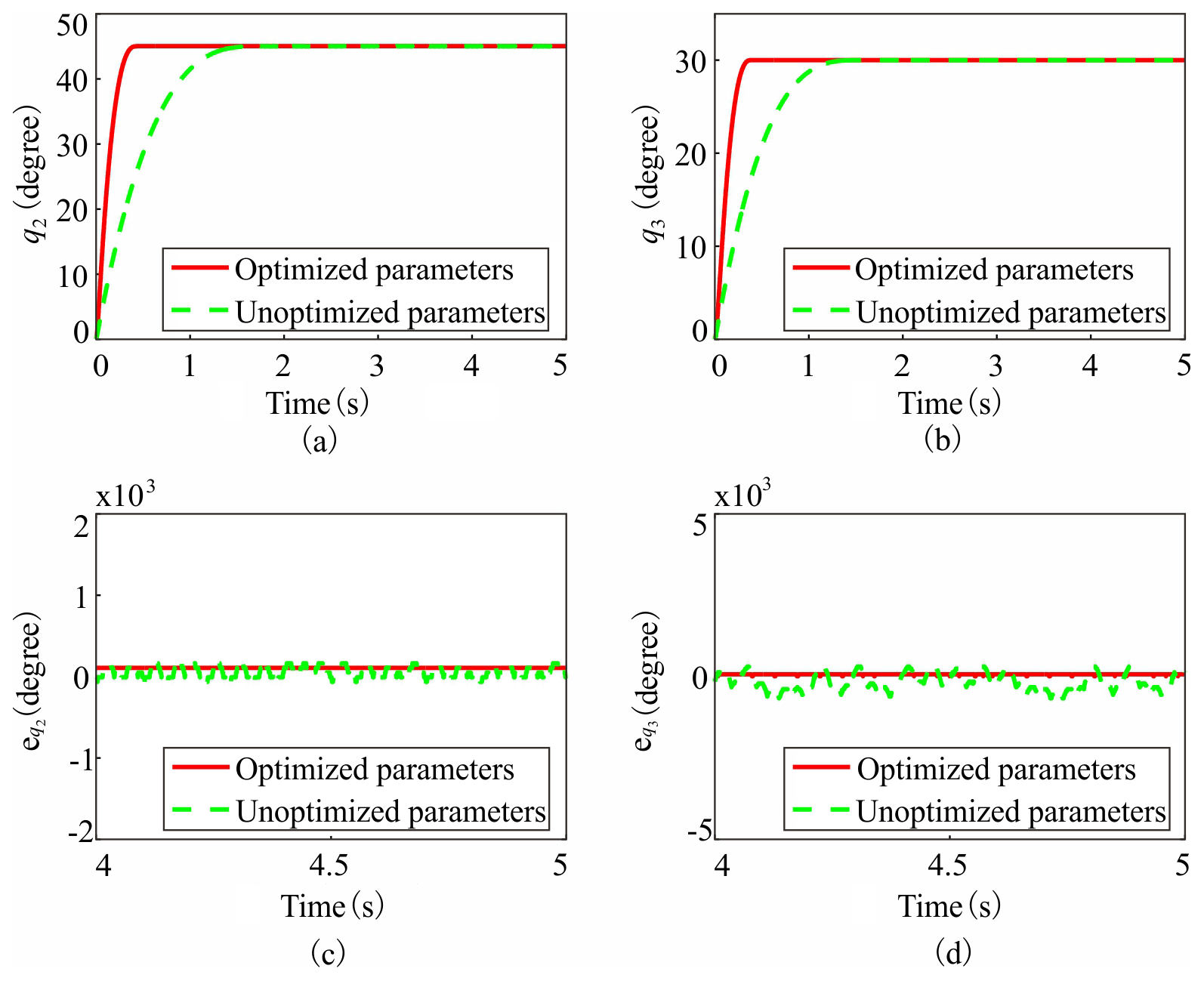
Figure 5 Numerical simulations of (a) q₂ and (b) q₃ responses in the two groups of control parameters. The corresponding steady-state error of (c) q₂ and (d) q₃.

4 Optimal-sliding-mode combined-control strategy

The optimal control input is designed to drive a dynamical system from an initial state to the predesigned terminal state so that a designed cost function reaches the extreme value (maximum or minimum). In the next section of this paper, the optimal control objective is set to make the cost function reach the minimum value. However, it is usually difficult to solve optimal control problems analytically for complex nonlinear dynamical systems. When the control input is bounded, even numerical optimal control solutions are quite difficult to obtain. That is an important factor that limits the application of optimal controls in engineering.

4.1 Algorithm

The cell mapping offers an efficient numerical way to solve optimal control problems. With the cell-mapping method, the continuum state space region is firstly discretized into a finite number of cells. Simultaneously, the bounded control inputs are also uniformly discretized. For each cell, the cell-to-cell mappings are constructed under different control input levels. Based on the constructed mapping database, the global optimal control solutions can be searched out. The cell-mapping method to deal with optimal control problems has universal applicability for linear and nonlinear dynamical systems. Moreover, it can ensure the global optimality of optimal control solutions as the search is instituted in the whole state space region. In addition, all the optimal control solutions of different controllable cells can be obtained, and uncontrollable cells can be recognized with one single run of the program.

The adjoining cell-mapping method, as an improvement of the simple cell-mapping method in dealing with optimal control problems, can construct the mapping database with smaller discretization error and can search the optimal control solution more efficiently. Furthermore, the closed-loop feedback control can be performed, which guarantees robustness in relation to the external disturbance. In the adjoining cell mapping, to deal with optimal control problems, the bounded external-control input is uniformly discretized as

$$\mathbf{U}=\left\{{\mathbf{u}}_{\mathrm{1}},{\mathbf{u}}_{\mathrm{2}},\mathrm{\dots },{\mathbf{u}}_{N_u}\right\},$$

where N_u is the total discretization number. Let z_i(n) represents the nth image cell of a previous image cell z_i(0); the one-step adjoining cell mapping can then be described as

$$\begin{array}{}\text{(15)}& {\mathbf{z}}_i\left(n\right)=C^{\mathrm{a}}\left({\mathbf{z}}_i\left(\mathrm{0}\right),{\mathbf{u}}_j\right).\end{array}$$

After the mapping database is constructed, the discrete optimal control table (DOCT) can be constructed by a back-stepping search strategy. As a result, every cell is assigned an optimal control input and an optimal cost function value. Those cells with the initial maximum index function value are recognized as uncontrollable cells.

Due to the existence of dimension disasters, the optimal control with the cell-mapping method is mainly applied in two-dimensional single-input–single-output system over quite a long time. The two-level subdivision strategy can make the cell-mapping method feasible to solve fixed-terminal-state optimal control problems for multi-input–multi-output (MIMO) systems. The state space region of interest can first be first discretized into relatively coarse cells, and the mapping database can then be constructed with GPU parallel technology. The optimal control inputs for all the controllable coarse cells can be searched for by means of the back-stepping search strategy, and the uncontrollable cells can be identified. Then the feedback control is instituted from a controllable initial state, and the integral trajectory starting from the initial coarse cell will cross several coarse cells in the state space before it reaches the cell where the target set is located. The region consisting of these continuous cells in the state space is further discretized, and the search is executed again to obtain the fine DOCT.

As for the trajectory-tracking optimal control problem, the target set is not fixed but is instead constantly changing over time. So the cell-mapping method to deal with fixed-terminal-state optimal control problems is no longer applicable. When the cell in which the target set is located changes, it is necessary to construct a new DOCT. Naturally, it is imagined that the target trajectory can be discretized into a series of points, namely, a series of cells in this paper. Then the trajectory-tracking optimal control problem can be transformed into a sequence of fixed-terminal-state optimal control problems, and the two-level subdivision strategy for the adjoining cell-mapping method can still be adopted to obtain optimal control solutions with a high computational efficiency. Based on this idea, a global optimal tracking control strategy with an adjoining cell-mapping method (OTCACM) is introduced (Tian et al., 2023). By using an adaptive criterion to judge the availability of adjoining cell-mapping pairs, the cell-mapping method is extended to solve optimal tracking control problems for MIMO systems for the first time.

However, it should be noted that the OTCACM may generate phase differences between the target trajectory and the system's real response trajectory. Before the target trajectory is cached up, the current system trajectory and the target trajectory are not in the same cell. Consequently, transformation of the trajectory-tracking optimal control to a sequence of fixed-terminal-state optimal controls is appropriate. However, after the current system trajectory and the target trajectory are in the same cell, real-time tracking for the target trajectory in the time domain is necessary to ensure a high control accuracy. It can be imagined that, on the one hand, if the target trajectory changes relatively slowly with time, the system response trajectory under optimal controls may shuttle back and forth around the target cell, which will result in the chattering phenomenon. The chattering amplitude and tracking error depend on the discretization scale of the state space region, namely, the size of cell; on the other hand, if the target trajectory changes relatively quickly with time, in some situations, such as the optimal control with minimum energy consumption, the resulting control input by OTCACM may be not insufficient to drive the system to catch the target cell quickly, which will result in the obvious phase lag phenomenon.

Based on the above analysis, an optimal and sliding-mode combined-control strategy (OSCC) is proposed. The OSCC employs the OTCACM law before the target trajectory is cached up and the ANTSMC law with optimized control parameters after the target trajectory is cached up. Let z_Φ represent the fine cell under the subdivision scale in which the current target state is located, while z_Δ is the cell in which the current target state is located. The OSCC can be described as

$$\begin{array}{}\text{(16)}& {\mathbf{u}}_{\mathrm{OSCC}}=\left\{\begin{array}{ll}{\mathbf{u}}_{\mathrm{OTCACM}},& {\mathbf{z}}_{\mathrm{\Delta }}\ne {\mathbf{z}}_{\mathrm{\Phi }}\\ {\mathbf{u}}_{\mathrm{ANTSMC}},& {\mathbf{z}}_{\mathrm{\Delta }}={\mathbf{z}}_{\mathrm{\Phi }}\end{array}\right..\end{array}$$

Note that the OSCC strategy combines the global optimality of the optimal control with cell mapping and the small steady-state tracking error of the sliding-mode control. With OSCC, a controlled system can be driven to catch up a target trajectory with the minimum cost function value and keep tracking for the target trajectory with a high accuracy after that.

Equation (16) means that the cells in which the current target state and system state are located need to be identified. If they are same, the ANTSMC law is adopted. If not, the OTCACM law is adopted. To detail the general procedure of OSCC, let M denote the database storing the information of all adjoining cell-mapping pairs described by Eq. (15), and let J denote the database storing the incremental cost function value J_ijk from a pre-image cell z_i in relation to its kth adjoining image cell under a control input u_j. If a cell can reach the target cell where the target trajectory is located in after the n-step adjoining cell mapping, it is denoted as an n-step controllable cell. The initial optimal control input ${\mathbf{u}}_i^{\ast }$ and the optimal cumulative cost function $J_i^{\ast }$ are assigned considerably large values. Those cells whose ${\mathbf{u}}_i^{\ast }$ and $J_i^{\ast }$ are never updated throughout are recognized as uncontrollable cells. The general procedure of OSCC is shown in Algorithm 1.

Algorithm 1 The general procedure of OSCC.

1:

Discretize the state space region into N_c cells

2:

Construct M and J in GPU

3:

Find the target cell. Set it as n-step controllable cell (n=0) and its cost function $J_i^{\ast }=\mathrm{0}$

4:

while (there is a cell whose $J_i^{\ast }$ can be updated to a smaller value) or (n<N_c) do

5:

Find all the mappings in M that enter into the n-step controllable cell and the corresponding incremental costs J_ijk from J. Calculate $J_i^{\ast }$ for every pre-image cell by adding J_ijk and $J_i^{\ast }$ of its image cell

6:

if ($J_i^{\ast }$ of a pre-image cell is smaller than before) then

7:

Update $J_i^{\ast }$ and ${\mathbf{u}}_i^{\ast }$

8:

$n=n+\mathrm{1}$. Set the cells whose $J_i^{\ast }$ and ${\mathbf{u}}_i^{\ast }$ are updated as n-step controllable cells

9:

end if

10:

end while

11:

The coarse cells crossed by the evolution trajectory from the current state to the target cell constitute a new region

12:

go to 1 so that the fine DOCT is constructed

13:

for (t=0 to T_e) do

14:

if (z_Δ=z_Φ) then

15:

Closed-loop feedback control with ANTSMC law

16:

else if (z_Δ≠z_Φ) then

17:

if (z_Φ remains unchanged) then

18:

The fine DOCT remains unchanged

19:

else if (z_Φ changes) and (the coarse target cell remain unchanged) then

20:

go to 3 so that a new fine DOCT is reconstructed

21:

else if (z_Φ changes) and (the coarse target cell changes) then

22:

go to 11 so that a new rough and fine DOCT are reconstructed

23:

end if

24:

Closed-loop feedback control under the fine DOCT

25:

end if

26:

end for

4.2 Simulations

Recalling the system in Eq. (1), the control target is set to drive the azimuth angle q₂ and pitch angle q₃ to track a sinusoidal motion with an amplitude of 30 degrees and a period of 5 s: $q_{\mathrm{20}}=q_{\mathrm{30}}=\mathrm{30}{}^{\circ }\left(\mathrm{2}\mathit{\pi }t/\mathrm{5}\right)$. The bounded state space region for $\left(q_{\mathrm{2}},{\dot{q}}_{\mathrm{2}},q_{\mathrm{3}},{\dot{q}}_{\mathrm{3}}\right)$ is set as $\left[-\mathrm{180}{}^{\circ },\mathrm{180}{}^{\circ }\right]\times \left[-\mathrm{6},\mathrm{6}\right]\times \left[-\mathrm{90}{}^{\circ },\mathrm{90}{}^{\circ }\right]\times \left[-\mathrm{3},\mathrm{3}\right]$ with the initial state $\left(-\mathrm{60}{}^{\circ },\mathrm{0},\mathrm{60}{}^{\circ },\mathrm{0}\right)$. The external-control torque inputs M₂ and M₃ are constrained in $\left[-\mathrm{25},\mathrm{25}\right]$. A quadratic index function which integrates control error and external energy consumption is set to estimate the optimal control performance:

$$\begin{array}{}\text{(17)}& J={\int }_{\mathrm{0}}^{T_{\mathrm{e}}}\left(a_{\mathrm{2}}{e}_{\mathrm{2}}^{\mathrm{2}}+b_{\mathrm{2}}{M}_{\mathrm{2}}^{\mathrm{2}}+a_{\mathrm{3}}{e}_{\mathrm{3}}^{\mathrm{2}}+b_c{M}_{\mathrm{3}}^{\mathrm{2}}\right)\mathrm{d}t,\end{array}$$

where $a_{\mathrm{2}}=a_{\mathrm{3}}=\mathrm{1}$, b₂=0.01, and b₃=0.025. The initial coarse discretization scale of the state space region is 31⁴, while the fine discretization scale is 5⁴. The external-control inputs M₂ and M₃ are uniformly dispersed with 50 levels each, which generates 2500 different control torque input combinations for (M₂,M₃). The construction of the cell-mapping database is instituted on the GPU device (NVIDIA GeForce GTX 1080Ti graphics card).

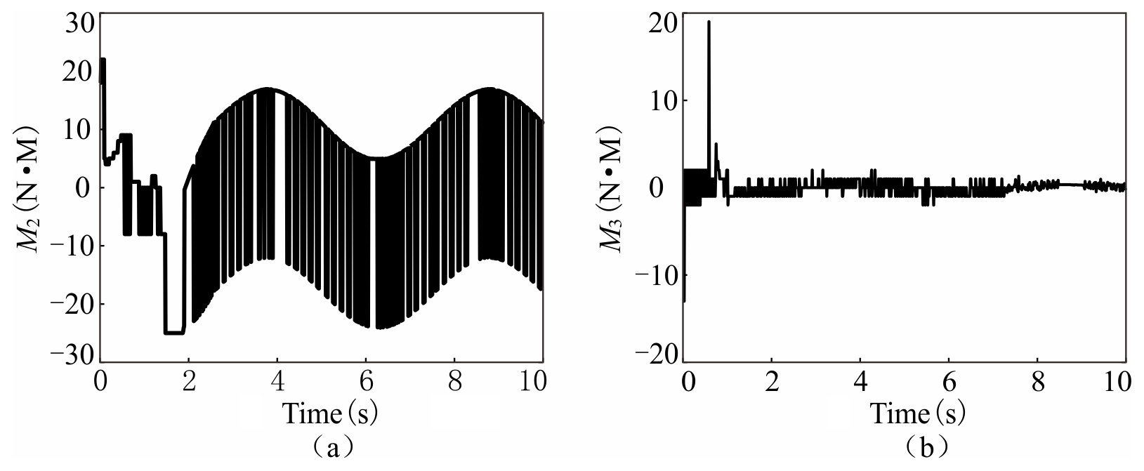
The feedback control evolution trajectories of q₂ and q₃ in the time domain under OSCC are shown in Fig. 6a and b. The dashed green and solid red lines represent the target trajectory and the real system response trajectory, respectively. It can be easily seen that both q₂ and q₃ catch up the target trajectories with the optimal performance index function and perform remarkable tracking with high control accuracy after that. The projections of the phase space evolution trajectory on 2D planes $\left(q_{\mathrm{2}},{\dot{q}}_{\mathrm{2}}\right)$ and $\left(q_{\mathrm{3}},{\dot{q}}_{\mathrm{3}}\right)$ are presented in Fig. 6c and d, respectively. After catching up the target ellipse trajectories in the phase space, the two practical trajectories coincide well with them. The control moment inputs M₂ and M₃ in the time domain under OSCC are shown in Fig. 7.

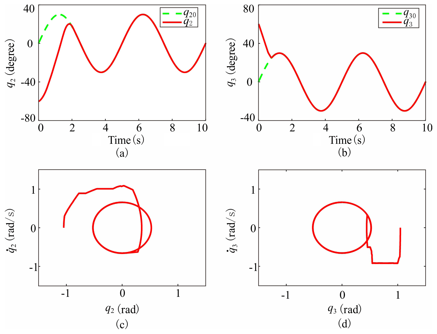
Figure 6 The feedback control evolution trajectories in the time domain under OSCC for (a) q₂ and (b) q₃. The projections of the phase space evolution trajectory on 2D planes (c) ($q_{\mathrm{2}},{\dot{q}}_{\mathrm{2}}$) and (d) ($q_{\mathrm{3}},{\dot{q}}_{\mathrm{3}}$).

Figure 7 The control moment inputs (a) M₂ and (b) M₃ in the time domain under OSCC.

For comparison, the feedback control evolution trajectories of q₂ and q₃ in the time domain under OTCACM (Tian et al., 2023) are exhibited in Fig. 8a and b. It is obvious that the tracking for q₂₀ almost fails due to the existence of serious phase lag, while the tracking for q₃₀ is effective. This happens as the cost function index described by Eq. (17) implies as small an input energy consumption as possible. Compared with the pitch turntable, the azimuth turntable possesses a relatively large moment of inertia. Therefore, the azimuth motor cannot drive the azimuth turntable to catch up the target trajectory timeously under the same control input level as the pitch motor. The projections of the phase space evolution trajectory on 2D planes $\left(q_{\mathrm{2}},{\dot{q}}_{\mathrm{2}}\right)$ and $\left(q_{\mathrm{3}},{\dot{q}}_{\mathrm{3}}\right)$ are presented in Fig. 8c and d, respectively. There exists a large deviation between the practical trajectory and the target elliptical trajectory on the $\left(q_{\mathrm{2}},{\dot{q}}_{\mathrm{2}}\right)$ plane. The chattering phenomenon is obvious in the tracking for q₃₀, which is due to the fact that the target trajectory changes relatively slowly with time. The phenomena of phase lag and chattering are consistent with the previous analysis.

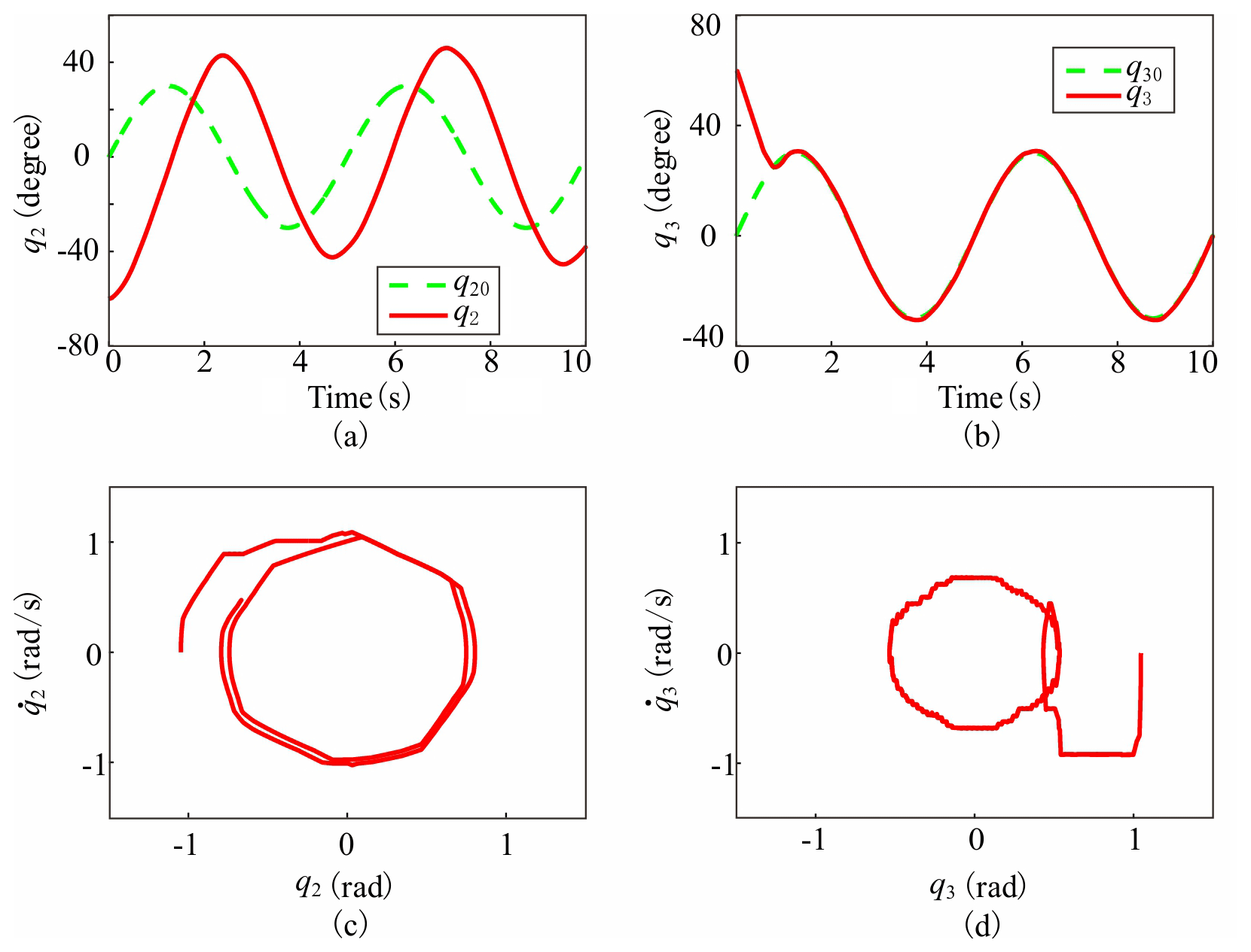
Figure 8 The feedback control evolution trajectories in time domain under OTCACM for (a) q₂ and (b) q₃. The projections of the phase space evolution trajectory on 2D planes (c) ($q_{\mathrm{2}},{\dot{q}}_{\mathrm{2}}$) and (d) ($q_{\mathrm{3}},{\dot{q}}_{\mathrm{3}}$).

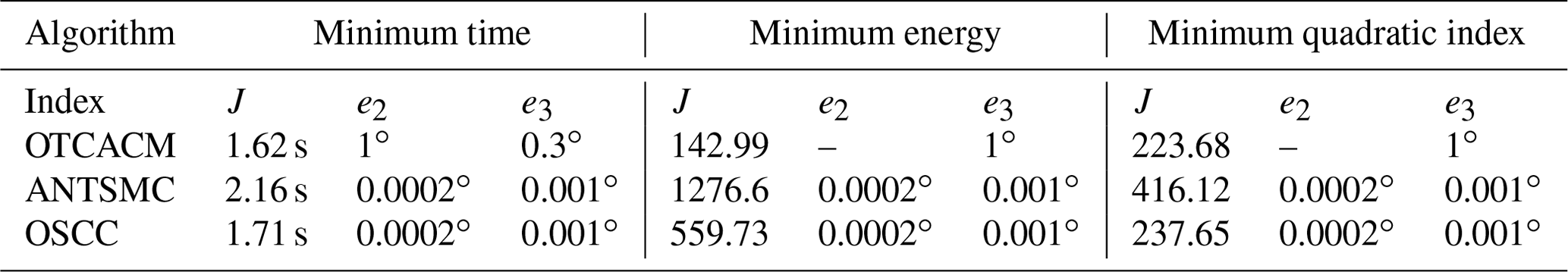
The minimum time, minimum energy consumption and minimum quadratic performance index tracking controls are instituted, respectively, for the antenna servo system with three different algorithms, namely, OTCACM, ANTSMC and OSCC. The comparisons of cost function value J and the steady errors e₂ and e₃ are shown in Table 3. The control accuracy increases obviously under OSCC compared with that under TCSCM, while the performance index function value decreases obviously under OSCC compared with that under ANTSMC.

Table 3 Control performance comparison of three control algorithms.

5 Conclusion

In this paper, the cell-mapping method is applied in the control optimization for an antenna servo system on a disturbed carrier.

To conquer the curse of dimensionality in the cell-mapping method for solving MOPs, the multi-parameter sensitivity analysis is implemented to realize the dimension reduction of the parameter space. A post-processing algorithm is also proposed to provide a reference in order for the decision maker to select proper control parameters from the Pareto set. The ANTSMC control parameters for the antenna servo system are optimized effectively with the proposed scheme. In addition, the OSCC strategy is introduced to overcome the tracking-phase difference phenomenon in the existing OTCACM. The OSCC combines the global optimality of optimal controls with cell mapping and the high tracking accuracy of the sliding-mode control. Simulation results show that, with the OSCC strategy, the antenna attitude angles are driven to catch up the target trajectories successfully with the global optimal cost function index and keep high accuracy tracking after that. The proposed approaches in this paper make the cell-mapping method more practical in the control optimization field, providing widely applicable and effective numerical solutions for control optimization problems for nonlinear dynamical systems in engineering.

Appendix A: Notation

B1	Vibration isolation equipment
B2	Azimuth turntable
B3	Pitch turntable
qi	Degrees of freedom for Bi
qi0	Target trajectory for qi
ei	Control error of qi
βi	Sliding-mode surface parameter for qi
γi	Sliding-mode surface parameter for qi
ki	Reaching-law parameter for qi
εi	Reaching-law parameter for qi
ci1	Reaching-law parameter for qi
ci2	Reaching-law parameter for qi
$O_{q_i}$	Overshoot of qi
$T_{{\mathrm{p}}_{q_i}}$	Peak time of qi
$E_{q_i}$	Steady-tracking error index of qi
E(Y | Xi)	Conditional expectation
V	Variance
ηi	Weight coefficient for MOP post-processing
zΦ	The fine cell in which the target state is located

zΔ	The fine cell in which the system state is located
Jijk	Incremental cost function from a pre-image cell zi in relation to its kth adjoining image cell under control input uj
${\mathbf{u}}_i^{*}$	Optimal control input for a cell zi
$J_i^{*}$	Optimal cumulative cost function for a cell zi
ANTSMC	Adaptive nonsingular terminal-sliding mode control
DOCT	Discrete optimal control table
LHS	Latin hypercube sampling
MIMO	Multi-input–multi-output
MOP	Multi-objective optimization problem
OSCC	Optimal-sliding mode combined control
OTCACM	Optimal tracking control with adjoining cell-mapping technology
SCM	Simple cell mapping