Ellipsoid contact analysis and application in the surface conjugate theory of face gears

The face gear tooth surface is a high-order variable curvature surface, and the curvature of the surface is complicated, so it is difficult to describe the characteristics of the face gear tooth surface by a specific equation. In this paper, the discrete curvature relation of the surface is used instead of an analytical equation to describe a spatial meshing surface, and the traditional meshing theory is neutralized to analyze the characteristics of the face gear tooth surface. Firstly, according to the structural characteristics of the face gear, the sampling method of the face gear tooth surface is analyzed, and the mathematical model of fitting the tooth surface contact point is established. Then, the discrete asymptotic surface development analysis method is studied, and the ellipsoid contact analysis method of the face gear pair is established by simplifying the conjugate surface and its region. Finally, the contact analysis method of the discrete tooth surface is studied, and the instantaneous contact ellipse of the face gear tooth surface is calculated, which formed a new numerical meshing method of space curved surface.

1 Introduction

The gear is the symbol of industrialization. The face gear is an advanced new configuration gear. The face gear transmission is a new type of advanced transmission that meshes with a kind of cylindrical spur gear and bevel gear. Compared with the traditional spiral bevel gear drive, it has the advantages of compact structure, small size, lightweight, high bearing capacity, high reliability, good interchangeability, no axial force, and remarkable processing efficiency, which can improve the transmission power and lifetime.

Face gear transmission has broad application prospects in the field of intersecting shaft power and motion transmission because of its simple structure, low vibration and noise, insensitivity to installation error, power split, and high interchangeability. NASA has funded projects such as the Advanced Rotor Program and the Rotorcraft Transmission Research Program (RDS-21), which have successfully applied face gear transmission technology to the power split device of a helicopter main reducer, greatly improving the overall performance of the transmission system. The face gear transmission technology has been successfully applied to the automotive power transmission system. Audi has successfully applied the face gear technology to the central differential, which reduces the weight compared to the traditional transmission mode and increases the torque distribution ratio between the front and rear wheels. In addition, the contribution ratio between the front and rear wheels has been improved. In addition, face gear transmission is also used in gear transmission systems such as reducers, dividing heads, high-end machine tools, radars, ships, fishing reels, and bicycle sprockets, and has achieved good results.

Gear meshing theory is the basis for face gear tooth surface forming; tooth contact analysis is performed to examine the meshing and bearing contact of the face gear pairs composed of a cylindrical spur gear and the bevel gear. Chang et al. (2000) derived the analytical geometry of the face gear drive and its mathematical model for tooth contact analysis of the face gear, as well as the spur pinion meshing. Litvin et al. (2002a, b) proposed an approach for design, tooth contact analysis, and stress analysis of formate-generated spiral bevel gears. And they also considered a face gear drive with a spur involute pinion; the generation of the face gear is based on the application of a grinding or cutting worm, whereas the conventional method of generation is based on the application of an involute shaper. Liu and Tsay (2002) investigated the contact characteristics of bevel gear pairs with intersected, crossed, and parallel axes. Guingand et al. (2005a, b) presented a procedure for analyzing the instantaneous loaded contact of a face gear and its experimental validation. And they further presented a method of simulating loaded face gear meshing. Tang and Liu (2013) introduced the analytical method based on Hertz theory on normal contact of elastic solids and the numerical method based on the finite-element method, calculating the contact stress of a face gear drive with spur involute pinion. To analyze the transmission performance of a face gear in real working conditions, Wang et al. (2012) investigated a calculation approach for load equivalent error of alignment to analyze the support system and tooth deformation of face gear drives. Lee (2016) proposed a cosine face gear, which is composed of a cosine pinion and a cosine face gear. According to the theory of conjugate tooth surfaces, they created the condition of undercutting for the cosine face gear.

He et al. (2017) obtained the mathematical model of the helical curve face gear and the tooth contact analysis. Li et al. (2017) proposed a face gear tooth modeling that is not based on conjugation theories, and they derived the extreme geometry boundary conditions of face gear teeth according to face gear tooth geometry characteristics. Based on the method of the principal curvatures of the space curve face, Lin et al. (2017) presented the loaded tooth contact analysis of the curve face gear pair. Wu et al. (2018) derived a method, based on the geometry characteristic of the tooth surface, to calculate the points as an even distribution on the tooth surface. Fu et al. (2018) proposed the application of a profile-shifted grinding disk to generate an offset, non-orthogonal and profile-shifted face gear. To solve the problem of the meshing efficiency of spur face gear sliding friction, Dong et al. (2018) proposed a gear based on elastohydrodynamic lubrication theory. Zhou et al. (2019) established an envelope method, according to the geometry characteristic of the shaper tooth surface, and the mathematical model of the face gear tooth surface can be represented as an explicit rather than an implicit one. Zschippang et al. (2000) elaborated on a method for the generation of a face gear with helix angle, shaft angle, and axle offset. Feng et al. (2019) investigated entire tooth surface precise modeling and systematic analysis method for face gear drives with an involute helical pinion. Liu and Zhang (2019) presented a spherical face gear pair by substituting the convex spherical gear for the pinion of a conventional face gear pair.

At present, the research on the meshing method of face gear transmission mainly focuses on coordinate transformation and formula derivation between the tool and target profile. Although some improvements have been made by optimizing the derivation process and transforming the boundary conditions, the induced curvature and other parameters cannot be accurately expressed in a specific equation. Given this, this paper presents data showing that the face gear tooth surface is expressed in the form of the second-order differential equation, and the meshing characteristics of the face gear complex surface can be analyzed by approximating the complex surface of the face gear. In the process of gear design, the visibility of the tooth surface contact state is poor, and finite-element calculation is complicated. There is a lack of unified calculation standards, and the results are difficult to control, making it difficult to guide machining. The long feedback period of face gear design, processing, and testing is seriously affected by the engineering application of a face gear.

Based on the abovementioned research, this paper proposes the digital tooth surface meshing theory of face gears, analyzes the discrete and sampling methods of the face gear surface, studies the analysis method of curvature of the spatial surface, and establishes the contact analysis method of space spheroid. The method can quickly define the tooth surface meshing performance of the face gear, which greatly shortens the face gear sub-design cycle. The design quality and stability are improved, and a foundation is laid for further engineering applications of face gears.

2 Tooth surface discretization and fitting

2.1 Discrete sampling

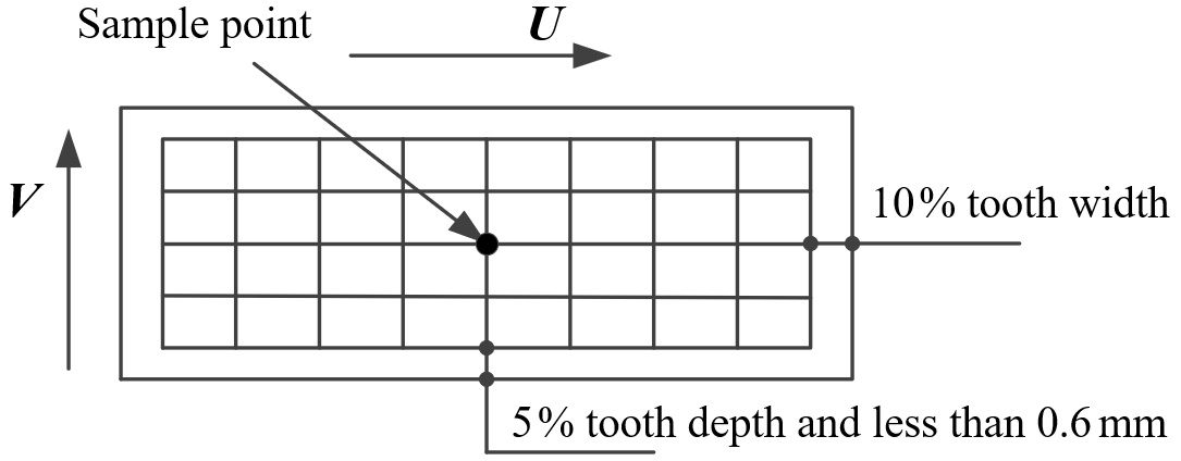
To analyze the meshing process of space-meshing digital teeth, this paper establishes a one-to-one correspondence between the measuring point and the space tooth surface equation. When selecting sampling points on the tooth surface or measuring the tooth surface with the coordinate measuring machine, the sampling points should be evenly distributed as far as possible. In general, 9 points are selected evenly in the direction of the teeth (U direction), and 5 points are selected evenly in the direction of the tooth width (V direction); 45 points are selected in total, and the grid intersection is shown in Fig. 1. This practice shows that if the selection is too few, it is not enough to reflect the shape of the tooth surface. However, if there are too many points, the sampling error of the sampling point may cause a local fluctuation of the tooth surface.

Figure 1 Tooth surface sampling diagram.

The meshing of the face gear tooth surface is shown in Fig. 2. For any grid node on the tooth surface, the distance r_grid from this point to the origin O₂ of the face gear coordinate system $S_{\mathrm{2}}(x_{\mathrm{2}},y_{\mathrm{2}},z_{\mathrm{2}})$ and the distance z_grid along the tooth height direction of the face gear can be expressed as

$$\begin{array}{}\text{(1)}& \left\{\begin{array}{l}{r}_{\mathrm{grid}}=\sqrt{r_{\mathrm{2}x}^{\mathrm{2}}+r_{\mathrm{2}y}^{\mathrm{2}}},\\ z_{\mathrm{grid}}=r_{\mathrm{2}z},\end{array}\right.\end{array}$$

where r_2x, r_2y, and r_2z are the components of the theoretical equation r₂(φ_s,θ_ks) of the face gear along the three directions of the coordinate system.

Figure 2 Schematic diagram of the grid point coordinate of a face gear.

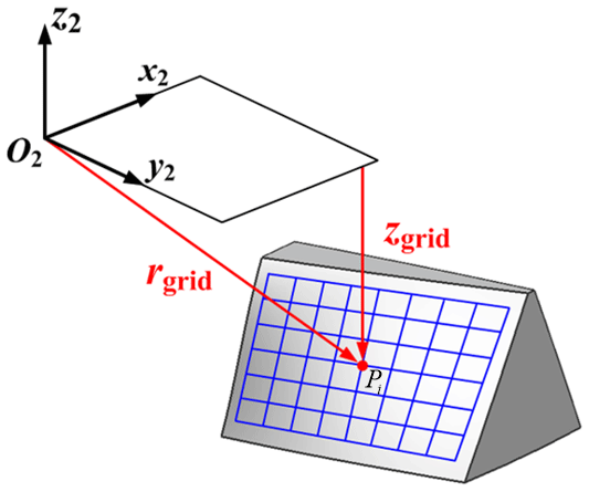
Equation (1) is a system of binary nonlinear equations about θ_ks and ϕ_s. For a face gear with given parameters, r_grid and z_grid are presented as numbers. Using the Newton iteration method to solve the above nonlinear equations, the coordinates $(x_{\mathrm{2}},y_{\mathrm{2}},z_{\mathrm{2}})$ and normal vectors $(n_{\mathrm{2}x},n_{\mathrm{2}y},n_{\mathrm{2}z})$ at each grid point of the face gear tooth surface can be calculated.

2.2 Establish the tooth surface fitting equation

The cubic B-spline function is used to fit the tooth surface sampling points, and the tooth surface fitting equation is obtained as follows:

$$\begin{array}{}\text{(2)}& {\mathit{S}}_i=\left[U_i\right]\left[\text{ms}\right]\left[{\mathit{O}}_{\mathbf{2}}{\mathit{P}}_{\mathit{i}}\right]\left[\text{mt}\right]\left[V_i\right],\end{array}$$

where

$$\begin{array}{rl}\left[U_i\right]& =\left[\begin{array}{cccc}{u}_i^{\mathrm{3}}& u_i^{\mathrm{2}}& u_i& \mathrm{1}\end{array}\right]\left(u_i\in [\mathrm{0},\mathrm{1}]\right),\\ \left[V_i\right]& =\left[\begin{array}{cccc}{v}_i^{\mathrm{3}}& v_i^{\mathrm{2}}& v_i& \mathrm{1}\end{array}\right]\left(v_i\in [\mathrm{0},\mathrm{1}]\right),\end{array}$$

$$\begin{array}{rl}\left[\text{ms}\right]& =\left[\begin{array}{cccc}-\mathrm{1}& \mathrm{3}& -\mathrm{3}& \mathrm{1}\\ \mathrm{3}& -\mathrm{6}& \mathrm{3}& \mathrm{0}\\ -\mathrm{3}& \mathrm{0}& \mathrm{3}& \mathrm{0}\\ \mathrm{1}& \mathrm{4}& \mathrm{1}& \mathrm{0}\end{array}\right],\\ \left[\text{mt}\right]& =\left[\begin{array}{cccc}-\mathrm{1}& \mathrm{3}& -\mathrm{3}& \mathrm{1}\\ \mathrm{3}& -\mathrm{6}& \mathrm{0}& \mathrm{4}\\ -\mathrm{3}& \mathrm{3}& \mathrm{3}& \mathrm{1}\\ \mathrm{1}& \mathrm{0}& \mathrm{0}& \mathrm{0}\end{array}\right].\end{array}$$

[O₂P_i] is a matrix of four rows and four columns of control points.

The control point is obtained by the type value point, and according to the geometrical invariance of the B-spline function, the coordinate transformation of the surface S_i is only performed by the coordinate transformation of its control point. Thus, the following formula can be obtained:

$$\begin{array}{}\text{(3)}& M{\mathit{S}}_i=\left[U_i\right]\left[\text{ms}\right]\left[{\mathit{O}}_{\mathbf{2}}{\mathit{P}}_{\mathit{i}}\right]\left[\text{mt}\right]\left[V_i\right].\end{array}$$

The surface normal vector N_i can be obtained as

$$\begin{array}{}\text{(4)}& {\mathit{N}}_i={\displaystyle \frac{{\mathit{S}}_{ui}^i\times {\mathit{S}}_{vi}^i}{\left|{\mathit{S}}_{ui}^i\times {\mathit{S}}_{vi}^i\right|}},\end{array}$$

where

$${\mathit{S}}_{ui}^i=\left[{\dot{U}}_i\right]\left[\text{ms}\right]\left|{\mathit{O}}_{\mathbf{2}}{\mathit{P}}_{\mathit{i}}\right|\left[\text{mt}\right]\left[V_i\right]$$

and ${\mathit{S}}_{vi}^i=\left[U_i\right]\left[\text{ms}\right]\left|{\mathit{O}}_{\mathbf{2}}{\mathit{P}}_{\mathit{i}}\right|\left[\text{mt}\right]\left[{\dot{V}}_i\right]$ are the tangent vectors in the U direction and V direction of the surface S_i at the point μ₁:

$$\left[{\dot{U}}_i\right]=\left[\begin{array}{cccc}\mathrm{3}{u}_i^{\mathrm{2}}& \mathrm{2}{u}_i& \mathrm{1}& \mathrm{0}\end{array}\right],\left[{\dot{V}}_i\right]=\left[\begin{array}{cccc}\mathrm{3}{v}_i^{\mathrm{2}}& \mathrm{2}{v}_i& \mathrm{1}& \mathrm{0}\end{array}\right].$$

2.3 Mathematical model of the tooth surface contact point

In Fig. 3, the solid line represents the situation of the instantaneous meshing contact between pinion 1 and face gear 2 at some point T in the space. As shown in Fig. 3, T₁ and T₂ are the points on the pinion and the face gear. R₁ and R₂ are the position vectors of the points T₁ and T₂ in each coordinate system, respectively. N₁ and N₂ are the unit normal vectors of the pinion and the face gear at these two points.

Figure 3 Face gear and pinion transmission.

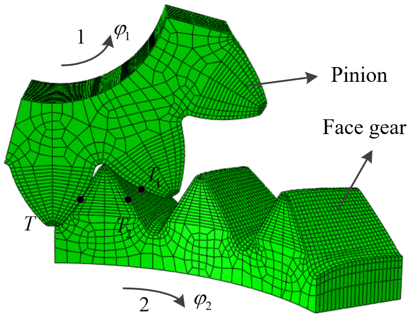
In establishing the solution model of the contact point, it can be assumed that pinion 1 is fixed in the coordinate system Σ₁. Suppose that when face gear 2 rotated φ₂ around its axis P, T₁ and T₂ would have instantaneous contact at point T, and we have

$$\begin{array}{}\text{(5)}& \left\{\begin{array}{l}{\mathit{R}}_{\mathrm{2}}=M\left({\mathit{\phi }}_{\mathrm{2}}{\mathit{P}}_{\mathrm{2}}\right)\otimes {\mathit{R}}_{\mathrm{2}},\\ {\mathit{N}}_{\mathrm{1}}=M\left({\mathit{\phi }}_{\mathrm{2}}{\mathit{P}}_{\mathrm{2}}\right)\otimes {\mathit{N}}_{\mathrm{1}},\end{array}\right.\end{array}$$

where (φ₂P₂)⊗R₂ represents when vector R₂ rotates φ₂ around the axis P₂. The equations consist of five equations with five unknowns (u₁, v₁, u₂, v₂, φ₂). For the convenience of further solution, Eq. (5) is converted. The following equation can be obtained:

$$\begin{array}{}\text{(6)}& \left\{\begin{array}{l}G\left(X\right)=min\left\{f\left(X\right)\right\},\\ \begin{array}{rl}f\left(X\right)=& \left|{\mathit{R}}_{\mathrm{1}}-M\left({\mathit{\phi }}_{\mathrm{2}}{\mathit{P}}_{\mathrm{2}}\right)\otimes {\mathit{R}}_{\mathrm{2}}\right|/\\ & \left(Q+\left|{\mathit{N}}_{\mathrm{1}}-M\left({\mathit{\phi }}_{\mathrm{2}}{\mathit{P}}_{\mathrm{2}}\right)\otimes {\mathit{N}}_{\mathrm{2}}\right|\right)\end{array},\\ x_j\in \left[a_j,b_j\right],\end{array}\right.\end{array}$$

where in $\left\{X\mathrm{|}{x}_j\left(j=\mathrm{0},\mathrm{1},\mathrm{\dots },\mathrm{4}\right)\right\}$ x_j stands for the five unknowns (u₁, v₁, u₂, v₂, φ₂); [a_j,b_j] is the corresponding interval for x_j; and |R| is the length of the vector R. Equation (6) transforms the problem of solving nonlinear equations in a certain interval into the minimum value optimization problem with constraints. In Eq. (6), Q(Q≥1) is introduced to reduce the influence of the position vector at the beginning of the search and to speed up the search. This is because in the initial search the change in the length of the position vector difference is not the same magnitude as the change in the length of the unit normal vector, and its value can be selected according to the specific situation.

When using this method to solve the contact point of the tooth surface, the pinion can be rotated around its axis P₁ to a certain meshing position and fixed; the surface parameters of the contact point and the rotation angle φ₂₀ of the large wheel at this moment can be solved. Then, the pinion in turn rotates Δφ₁ around its axis P₁, and it solves the rotation φ₂ of the face gear and calculates the angle increment $\mathrm{\Delta }{\mathit{\phi }}_{\mathrm{2}}={\mathit{\phi }}_{\mathrm{2}}^{\prime }-{\mathit{\phi }}_{\mathrm{20}}$ of the face gear.

Suppose that the pinion is rotated around the axis P₁ by angle Δφ₁, then the tooth surface equation is ${{\mathit{S}}^{\mathbf{\prime }}}_{\mathrm{1}}$. The one corresponding to the angle of increment of a face gear is Δφ₂, and the face gear tooth surface equation is ${{\mathit{S}}^{\mathbf{\prime }}}_{\mathrm{2}}$. The tooth surfaces ${{\mathit{S}}^{\mathbf{\prime }}}_{\mathrm{1}}$ and ${{\mathit{S}}^{\mathbf{\prime }}}_{\mathrm{2}}$ contact at point T^′, and the first-class basic quantity of the tooth surface ${{\mathit{S}}^{\mathbf{\prime }}}_{\mathrm{1}}$ and ${{\mathit{S}}^{\mathbf{\prime }}}_{\mathrm{2}}$ are given as

$$\begin{array}{}\text{(7)}& E_i={{\mathit{S}}^{\mathbf{\prime }}}_{ui}^{\mathrm{2}},F_i={{\mathit{S}}^{\mathbf{\prime }}}_{ui}\cdot {{\mathit{S}}^{\mathbf{\prime }}}_{ui}^{\prime },G_i={{\mathit{S}}^{\mathbf{\prime }}}_{vi}^{\mathrm{2}}.\end{array}$$

The second-class basic quantity is expressed as follows:

$$\begin{array}{}\text{(8)}& L_i=N_i\cdot {{\mathit{S}}^{\mathbf{\prime }}}_{uui},M_i=\mathit{n}\cdot {{\mathit{S}}^{\mathbf{\prime }}}_{uvi},G_i=n{{\mathit{S}}^{\mathbf{\prime }}}_{vvi},\end{array}$$

where n is the normal vector at point $T_c^{\prime }$; ${{\mathit{S}}^{\mathbf{\prime }}}_{ui}$ is the first derivative of the tooth surface i on the parameter u_i; and ${{\mathit{S}}^{\mathbf{\prime }}}_{uvi}$ is the second derivative of the tooth surface i on the parameter u_i.

3 Curvature analysis of space monolithic free-form surface

The binary vector function r(u,v) has two parameters u and v. When u and v change, its endpoint M will draw a continuous surface S in space, and its equation can be expressed as

$$\begin{array}{}\text{(9)}& r(u,v)=\left(x(u,v),y(u,v),z(u,v)\right).\end{array}$$

Suppose that M₀ is any point on the surface S, and its surface coordinates are u₀ and v₀. If we let v=v₀ and only change u, we can get a curve $r=r(u,v_{\mathrm{0}})$ passing through M₀ on the surface S. Similarly, if we let u=u₀ and only change v in Eq. (1), we can get a curve $r=r(u_{\mathrm{0}},v)$ passing through M₀ on the surface S. According to the properties of the space surface, we can solve the first-order and second-order partial derivatives.

$$\begin{array}{}\text{(10)}& \begin{array}{rl}{r}_u\left(u_{\mathrm{0}},v_{\mathrm{0}}\right)& ={\displaystyle \frac{\partial r\left(u_{\mathrm{0}},v_{\mathrm{0}}\right)}{\partial u}},r_v\left(u_{\mathrm{0}},v_{\mathrm{0}}\right)={\displaystyle \frac{\partial r\left(u_{\mathrm{0}},v_{\mathrm{0}}\right)}{\partial v}},\\ r_{uu}\left(u_{\mathrm{0}},v_{\mathrm{0}}\right)& ={\displaystyle \frac{{\partial }^{\mathrm{2}}r\left(u_{\mathrm{0}},v_{\mathrm{0}}\right)}{\partial u^{\mathrm{2}}}},r_{uv}\left(u_{\mathrm{0}},v_{\mathrm{0}}\right)={\displaystyle \frac{{\partial }^{\mathrm{2}}r\left(u_{\mathrm{0}},v_{\mathrm{0}}\right)}{\partial u\partial v}},\\ r_{vv}\left(u_{\mathrm{0}},v_{\mathrm{0}}\right)& ={\displaystyle \frac{{\partial }^{\mathrm{2}}r\left(u_{\mathrm{0}},v_{\mathrm{0}}\right)}{\partial v^{\mathrm{2}}}}.\end{array}\end{array}$$

The first fundamental homogeneous equation of the surface is expressed as follows:

$$\begin{array}{}\text{(11)}& \mathrm{d}{s}^{\mathrm{2}}=E\mathrm{d}{u}^{\mathrm{2}}+\mathrm{2}F\mathrm{d}u\mathrm{d}v+G\mathrm{d}{v}^{\mathrm{2}},\end{array}$$

where E, F, and G are the coefficients of the first fundamental homogeneous equation, respectively.

$$E=(r_u{)}^{\mathrm{2}},F=r_u{r}_v,G=(r_v{)}^{\mathrm{2}}.$$

The second fundamental homogeneous equation of the surface is expressed as follows:

$$\begin{array}{}\text{(12)}& \mathit{\phi }=L\mathrm{d}{u}^{\mathrm{2}}+\mathrm{2}M\mathrm{d}u\mathrm{d}v+N\mathrm{d}{v}^{\mathrm{2}},\end{array}$$

where L, M, and N are the coefficients of the second fundamental homogeneous equation, respectively.

$$\begin{array}{}\text{(13)}& L=n{r}_{uu},M=n{r}_{uv},N=n{r}_{vv}.\end{array}$$

The unit normal vector of surface S at M₀ is expressed as follows:

$$\begin{array}{}\text{(14)}& n={\displaystyle \frac{r_u\times r_v}{\left|r_u\times r_v\right|}}.\end{array}$$

Substituting the coefficient of the first fundamental homogeneous equation into Eq. (14), then

$$\begin{array}{}\text{(15)}& n={\displaystyle \frac{r_u\times r_v}{\sqrt{EG-F^{\mathrm{2}}}}}.\end{array}$$

The normal curvature k_n of the surface is expressed as follows:

$$\begin{array}{}\text{(16)}& k_n=n{\displaystyle \frac{d^{\mathrm{2}}r}{\mathrm{d}{s}^{\mathrm{2}}}}=k\mathit{\beta }n=k\cos \mathit{\theta },\end{array}$$

where β is the main normal vector, and k is the curvature of the curve r at M₀; θ is the angle between β and n.

Substituting the coefficients of the first basic homogeneous form and the second basic homogeneous form, the formula for calculating the normal curvature is expressed as follows:

$$\begin{array}{}\text{(17)}& k_n={\displaystyle \frac{L\mathrm{d}{u}^{\mathrm{2}}+\mathrm{2}M\mathrm{d}u\mathrm{d}v+N\mathrm{d}{v}^{\mathrm{2}}}{E\mathrm{d}{u}^{\mathrm{2}}+\mathrm{2}F\mathrm{d}y\mathrm{d}v+G\mathrm{d}{v}^{\mathrm{2}}}}.\end{array}$$

The torsion of curvature at points M along $\mathit{\alpha }=\frac{\mathrm{d}r}{\mathrm{d}s}$ is expressed as follows:

$$\begin{array}{}\text{(18)}& {\mathit{\tau }}_g=-\left({\displaystyle \frac{\mathrm{d}n}{\mathrm{d}s}},n,{\displaystyle \frac{\mathrm{d}r}{\mathrm{d}s}}\right).\end{array}$$

We introduce the coefficients of the first and second fundamental homogeneous equations to obtain the calculation formula for the short-range torsion rate.

$$\begin{array}{}\text{(19)}& \begin{array}{rl}& {\mathit{\tau }}_g\\ & ={\displaystyle \frac{(EM-FL)\mathrm{d}{u}^{\mathrm{2}}+(EN-GL)\mathrm{d}u\mathrm{d}v+(FN-GM)\mathrm{d}{v}^{\mathrm{2}}}{\sqrt{EF-G^{\mathrm{2}}}\left(E\mathrm{d}{u}^{\mathrm{2}}+\mathrm{2}F\mathrm{d}u\mathrm{d}v+G\mathrm{d}{v}^{\mathrm{2}}\right)}}\end{array}\end{array}$$

Then, we have

$$\begin{array}{}\text{(20)}& {\mathit{\tau }}_g={\displaystyle \frac{\mathrm{1}}{\mathrm{2}}}{\displaystyle \frac{\mathrm{d}{k}_n}{\mathrm{d}\mathit{\theta }}}.\end{array}$$

Let g₁ and g₂ be the main directions. The principal curvature of direction g₁ is k₁, and the principal curvature in the direction g₂ is k₂. The angle between α and g₁ is θ. According to the Euler formula and the Bertrand formula, we have the following:

$$\begin{array}{}\text{(21)}& \begin{array}{rl}{k}_n& =k_{\mathrm{1}}{\cos }^{\mathrm{2}}\mathit{\theta }+k_{\mathrm{2}}{\sin }^{\mathrm{2}}\mathit{\theta }={\displaystyle \frac{k_{\mathrm{1}}+k_{\mathrm{2}}}{\mathrm{2}}}+{\displaystyle \frac{k_{\mathrm{1}}-k_{\mathrm{2}}}{\mathrm{2}}}\cos \mathrm{2}\mathit{\theta },\\ {\mathit{\tau }}_g& =-\left(k_{\mathrm{1}}-k_{\mathrm{2}}\right)\sin \mathit{\theta }\cos \mathit{\theta }=-{\displaystyle \frac{k_{\mathrm{1}}-k_{\mathrm{1}}}{\mathrm{2}}}\sin \mathrm{2}\mathit{\theta }.\end{array}\end{array}$$

Set the angle between α₁ and g₁ to φ, and the angle between α₂ and g₁ to 90^∘ +φ. From Eq. (21), the normal curvature and short-range torsion of the α₁ direction and the α₂ direction are expressed as follows:

$$\begin{array}{}\text{(22)}& \begin{array}{rl}{k}_{n\mathrm{1}}& ={\displaystyle \frac{k_{\mathrm{1}}+k_{\mathrm{2}}}{\mathrm{2}}}+{\displaystyle \frac{k_{\mathrm{1}}-k_{\mathrm{2}}}{\mathrm{2}}}\cos \mathrm{2}\mathit{\phi },\\ k_{n\mathrm{1}}& ={\displaystyle \frac{k_{\mathrm{1}}+k_{\mathrm{2}}}{\mathrm{2}}}-{\displaystyle \frac{k_{\mathrm{1}}-k_{\mathrm{2}}}{\mathrm{2}}}\cos \mathrm{2}\mathit{\phi },\\ {\mathit{\tau }}_g& =-{\displaystyle \frac{k_{\mathrm{1}}-k_{\mathrm{2}}}{\mathrm{2}}}\sin \mathrm{2}\mathit{\phi }.\end{array}\end{array}$$

When we substitute them to k_n1k_n2−(τ_g1)², we have the following:

$$\begin{array}{}\text{(23)}& k_{n\mathrm{1}}{k}_{n\mathrm{2}}-({\mathit{\tau }}_{g\mathrm{1}}{)}^{\mathrm{2}}=k_{\mathrm{1}}{k}_{\mathrm{2}}.\end{array}$$

According to the above basic formula of the surface, the curvature characteristics of the space free surface are analyzed. The simulation results of the face gear are shown in Fig. 4.

Figure 4 Direction distribution diagram of the main curvature of the face gear.

4 Generative analysis of the discrete curvature asymptotic surface

4.1 Curvature of the conjugate surface

Knowing two surfaces, when solving the conjugate motion relationship of the surfaces in the contact process, the average curvature and Gaussian curvature are used to describe the characteristics of the points on the surface. We suppose that the two curvatures are denoted by k₁ and k₂ and are determined by the following equations.

$$\begin{array}{}\text{(24)}& \begin{array}{rl}H& ={\displaystyle \frac{k_{\mathrm{1}}+k_{\mathrm{2}}}{\mathrm{2}}}={\displaystyle \frac{EN-\mathrm{2}FM+GL}{\mathrm{2}\left(EG-F^{\mathrm{2}}\right)}},\\ K& =k_{\mathrm{1}}{k}_{\mathrm{2}}={\displaystyle \frac{LN-M^{\mathrm{2}}}{EG-F^{\mathrm{2}}}},\end{array}\end{array}$$

where E, F, and G are the first fundamental quantities of the surface, and L, M, and N are the second fundamental quantities of the surface.

The average curvature H is a key indicator of curvature, and the Euler equation can prove that the average value of normal curvature of a point on the surface along two orthogonal directions is the same; it equals the average curvature. This shows that the curvature of a point only considers average curvature. Therefore, when the regional structure is simplified, the substituted constructed surfaces must have equal Gaussian curvature and mean curvature. In other words, it should have the same principal curvature and main direction. In some simple secondary, rotating surfaces, such as ellipsoids, cylinders, and hyperboloids, the longitude lines and latitude lines are geodesics, and the measuring torque is zero. Therefore, the direction of the longitude line and latitude line becomes the main direction and the main curvature, which can replace the conjugate surface contact area.

4.2 Equations and expressions of the ellipsoid

According to the surface feature of the initial point, the surface can be simplified to the elliptical surface, cylindrical surface, and hyperboloid; all three types can be written as general statements.

$$\begin{array}{}\text{(25)}& x^{\mathrm{2}}+f{y}^{\mathrm{2}}+z^{\mathrm{2}}=a^{\mathrm{2}}\end{array}$$

In the equation, $f=\pm \frac{a^{\mathrm{2}}}{b^{\mathrm{2}}}$, and a and b are the lengths of the long axis and the short axis, respectively.

And this assumes b≥a, so

$$\begin{array}{}\text{(26)}& -\mathrm{1}\le f\le \mathrm{1}.\end{array}$$

When $-\mathrm{1}\le f\le \mathrm{0}$, it is a hyperbola.
When $-f=\mathrm{0}$, it is a circular cylinder with a radius of a.
When $\mathrm{0}\le f\le \mathrm{1}$, it is the rotation of the ellipse.

Suppose that these three types of surfaces are all rotating surfaces with the Y axis as the rotation axis; the longitude line as a circle; and the latitude line as an elliptical spiral, a straight line, or a hyperbola, respectively. The normal of the ellipsoid is N=[x fy z]^T, and its direction points to the outside; the normal curvature of the longitude line and the latitude line of the ellipsoid are given as

$$\begin{array}{}\text{(27)}& \left\{\begin{array}{l}{k}_g=\frac{-f{a}^{\mathrm{2}}}{{\left[a^{\mathrm{2}}+f^{\mathrm{2}}{y}^{\mathrm{2}}-f{y}^{\mathrm{2}}\right]}^{\frac{\mathrm{3}}{\mathrm{2}}}},\\ k_t={\displaystyle \frac{-\mathrm{1}}{\sqrt{a^{\mathrm{2}}+f^{\mathrm{2}}{y}^{\mathrm{2}}-f{y}^{\mathrm{2}}}}}.\end{array}\right.\end{array}$$

4.3 Replacement of the conjugate surface with an ellipsoid

When a point P=[a 0 0]^T on the surface of the ellipsoid matches a point on the conjugate surface, its normal direction should be the same as the fixed point. The main direction of P is the same as that of the specified point on the conjugate surface, and the principal curvature is equal. According to the characteristics of the ellipsoid, the two main directions of the P points should be the longitude line and the latitude line, and the normal curvature of the longitude line and latitude line should be

$$\begin{array}{}\text{(28)}& \left\{\begin{array}{l}{k}_g=-f/a,\\ k_t=-\mathrm{1}/a.\end{array}\right.\end{array}$$

However, the absolute value of two normal curvatures is expressed as $\left|k_g\right|=a/b^{\mathrm{2}}$ and $\left|k_t\right|=\mathrm{1}/a$. Because b≥a, so $\left|k_g\right|\le \left|k_t\right|$. This shows that the y axis is usually the long axis of the ellipsoid. It is assumed that the two main curvatures on the conjugate surface have the following relation: $\left|k_{\mathrm{1}}\right|\le \left|k_{\mathrm{2}}\right|$. When the ellipsoid replaces the hyperboloid, i.e., k_g=k₁ and k_t=k₂, we can deduce that $a=-\mathrm{1}/k_{\mathrm{2}}$ and $f=k_{\mathrm{1}}/k_{\mathrm{2}}$.

5 Ellipsoid contact analysis (ECA)

After the ellipsoid replaces the conjugate surface, the problem of solving conjugate surfaces becomes the problem of solving the minimum distance between two points. Suppose that the two ellipsoids S₁ and S₂ are placed in two coordinate systems σ₁(O₁−x₁y₁z₁) and σ₂(O₂−x₂y₂z₂), and S₁ and S₂ can be, respectively, expressed as follows:

$$\begin{array}{}\text{(29)}& \left\{\begin{array}{l}{x}_{\mathrm{1}}^{\mathrm{2}}+f_{\mathrm{1}}{y}_{\mathrm{1}}^{\mathrm{2}}+z_{\mathrm{1}}^{\mathrm{2}}=a_{\mathrm{1}}^{\mathrm{2}},\\ x_{\mathrm{2}}^{\mathrm{2}}+f_{\mathrm{2}}{y}_{\mathrm{2}}^{\mathrm{2}}+z_{\mathrm{2}}^{\mathrm{2}}=a_{\mathrm{2}}^{\mathrm{2}}.\end{array}\right.\end{array}$$

The normal vector of the ellipsoid can be expressed as

$$\begin{array}{}\text{(30)}& \left\{\begin{array}{l}{N}_{\mathrm{1}}={\left[\begin{array}{ccc}{x}_{\mathrm{1}}& f_{\mathrm{1}}{y}_{\mathrm{1}}& z_{\mathrm{1}}\end{array}\right]}^T,\\ N_{\mathrm{2}}={\left[\begin{array}{ccc}{x}_{\mathrm{2}}& f_{\mathrm{2}}{y}_{\mathrm{2}}& z_{\mathrm{2}}\end{array}\right]}^T.\end{array}\right.\end{array}$$

5.1 Minimum distance between ellipsoid and ellipsoid

Assume that the rotation matrix from σ₂ to σ₁ is expressed as follows:

$$\begin{array}{}\text{(31)}& M=\left[\begin{array}{ccc}{M}_{\mathrm{11}}& M_{\mathrm{12}}& M_{\mathrm{13}}\\ M_{\mathrm{21}}& M_{\mathrm{22}}& M_{\mathrm{23}}\\ M_{\mathrm{31}}& M_{\mathrm{32}}& M_{\mathrm{33}}\end{array}\right].\end{array}$$

The vector between two coordinate centers (two ellipsoid centers) can be expressed as

$$\begin{array}{}\text{(32)}& \mathit{\rho }={\mathit{O}}_{\mathbf{1}}{\mathit{O}}_{\mathbf{2}}=\left[\begin{array}{ccc}{\mathit{\rho }}_x& {\mathit{\rho }}_y& {\mathit{\rho }}_z\end{array}\right].\end{array}$$

Based on the conjugate theory, the two points with the minimum distance are usually on two conjugate surfaces, the normal lines of the two points are parallel to each other, and the vectors between the two points are parallel to the normal line. Therefore, we have

$$\begin{array}{}\text{(33)}& \left\{\begin{array}{l}{K}_n{N}_l=M{N}_{\mathrm{2}},\\ K_r{N}_l=M{r}_{\mathrm{2}}-r_{\mathrm{1}}+p,\end{array}\right.\end{array}$$

where K_n and K_r are two unknown coefficients that can be expressed as

$$\begin{array}{}\text{(34)}& \left\{\begin{array}{l}{K}_n{x}_{\mathrm{1}}=M_{\mathrm{11}}{x}_{\mathrm{2}}+M_{\mathrm{12}}{f}_{\mathrm{2}}{y}_{\mathrm{2}}+M_{\mathrm{13}}{z}_{\mathrm{2}},\\ K_n{f}_{\mathrm{1}}{y}_{\mathrm{1}}=M_{\mathrm{21}}{x}_{\mathrm{2}}+M_{\mathrm{22}}{f}_{\mathrm{2}}{y}_{\mathrm{2}}+M_{\mathrm{23}}{z}_{\mathrm{2}},\\ K_n{z}_{\mathrm{1}}=M_{\mathrm{31}}{x}_{\mathrm{2}}+M_{\mathrm{32}}{f}_{\mathrm{2}}{y}_{\mathrm{2}}+M_{\mathrm{33}}{z}_{\mathrm{2}},\\ K_r{x}_{\mathrm{1}}=M_{\mathrm{11}}{x}_{\mathrm{2}}+M_{\mathrm{12}}{y}_{\mathrm{2}}+M_{\mathrm{13}}{z}_{\mathrm{2}}-x_{\mathrm{1}}+{\mathit{\rho }}_x,\\ K_r{f}_{\mathrm{1}}{y}_{\mathrm{1}}=M_{\mathrm{21}}{x}_{\mathrm{2}}+M_{\mathrm{22}}{y}_{\mathrm{2}}+M_{\mathrm{23}}{z}_{\mathrm{2}}-y_{\mathrm{1}}+{\mathit{\rho }}_y,\\ K_r{z}_{\mathrm{1}}=M_{\mathrm{31}}{x}_{\mathrm{2}}+M_{\mathrm{32}}{y}_{\mathrm{2}}+M_{\mathrm{33}}{z}_{\mathrm{2}}-z_{\mathrm{1}}+{\mathit{\rho }}_z.\end{array}\right.\end{array}$$

The minimum distance between two points can be obtained from the eight equations (Eqs. 32 and 34). To obtain the analytical solution, the hypothesis of the ellipsoid should be further simplified.

5.2 Analytical solution from point to ellipsoid

The ellipsoid S₂ is simplified to a point, where x₂, y₂, and z₂ are zero. According to the above derivation, we can obtain

$$\begin{array}{}\text{(35)}& \left\{\begin{array}{l}\left(K_r+\mathrm{1}\right)x_{\mathrm{1}}={\mathit{\rho }}_x,\\ \left(K_r{f}_{\mathrm{1}}+\mathrm{1}\right)y_{\mathrm{1}}={\mathit{\rho }}_y,\\ \left(K_r+\mathrm{1}\right)z_{\mathrm{1}}={\mathit{\rho }}_z.\end{array}\right.\end{array}$$

This can be obtained by substituting Eq. (35) into Eq. (32).

$$\begin{array}{}\text{(36)}& D_{\mathrm{1}}{K}_r^{\mathrm{4}}+D_{\mathrm{2}}{K}_r^{\mathrm{3}}+D_{\mathrm{3}}{K}_r^{\mathrm{2}}+D_{\mathrm{4}}{K}_r+D_{\mathrm{5}}=\mathrm{0},\end{array}$$

where

$$\begin{array}{l}{D}_{\mathrm{1}}=-a_{\mathrm{1}}^{\mathrm{2}}{f}_{\mathrm{1}}^{\mathrm{2}},\\ D_{\mathrm{2}}=-\mathrm{2}{a}_{\mathrm{1}}^{\mathrm{2}}{f}_{\mathrm{1}}\left(\mathrm{1}-f_{\mathrm{1}}\right),\\ D_{\mathrm{3}}={\mathit{\rho }}_x^{\mathrm{2}}{f}_{\mathrm{1}}^{\mathrm{2}}+f_{\mathrm{1}}{\mathit{\rho }}_y^{\mathrm{2}}+{\mathit{\rho }}_z^{\mathrm{2}}{f}_{\mathrm{1}}^{\mathrm{2}}-a_{\mathrm{1}}^{\mathrm{2}}\left(\mathrm{1}+\mathrm{4}{f}_{\mathrm{1}}+f_{\mathrm{1}}^{\mathrm{2}}\right),\\ D_{\mathrm{4}}=\mathrm{2}\left[\left({\mathit{\rho }}_{x\mathrm{1}}^{\mathrm{2}}+{\mathit{\rho }}_y^{\mathrm{2}}+{\mathit{\rho }}_z^{\mathrm{2}}\right)f_{\mathrm{1}}-a_{\mathrm{1}}^{\mathrm{2}}-a_{\mathrm{1}}^{\mathrm{2}}{f}_{\mathrm{1}}\right],\\ D_{\mathrm{5}}={\mathit{\rho }}_x^{\mathrm{2}}+f_{\mathrm{1}}{\mathit{\rho }}_y^{\mathrm{2}}+{\mathit{\rho }}_z^{\mathrm{2}}-a_{\mathrm{1}}^{\mathrm{2}}.\end{array}$$

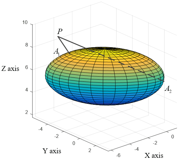
Four analytical solutions can be obtained from Eq. (36), two of which are real solutions and the other two are imaginary solutions. Figure 5 shows the diagram of the real solution. The imaginary solution shown in Fig. 6 should be given up. The two real solutions are the nearest A₁ and the farthest A₂ from P. Get rid of the farthest point according to the requirements. Then, point A₁ of the analytical solution is obtained, which is the closest point of the ellipse to P.

Figure 5 Diagram of the real solution.

Figure 6 Schematic diagram of finite iteration.

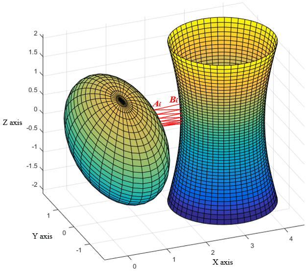
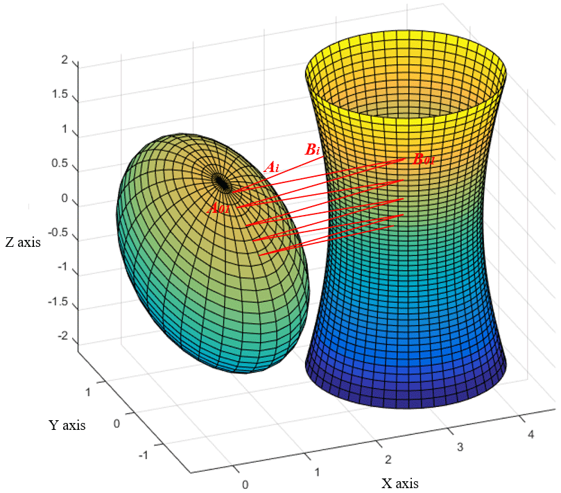
After obtaining the A₁ point on the ellipsoid, the shortest distance point B₁ from A₁ to S₂ can be solved by repeating the solution of the four polynomials of A₁ to the ellipsoid S₂. Thus, an iterative process is completed. Figure 6 shows the points A_i and B_i that have been iterated over six times. The minimum distance can be obtained through finite iteration and the iteration termination condition.

$$\begin{array}{}\text{(37)}& \begin{array}{rl}& \left|r_{Ai}-r_{Bi}\right|-\left|r_{A(i-\mathrm{1})}-r_{B(i-\mathrm{1})}\right|\le {\mathit{\epsilon }}_{\mathrm{1}},\\ & \left|N_{Ai}\times N_{Bi}\right|\le {\mathit{\epsilon }}_{\mathrm{2}},\end{array}\end{array}$$

where ε₁ and ε₂ represent the convergence precision.

5.3 The analytical solution of the ball to the ellipsoid

The main reason for the low solution speed is that the ellipsoid surface features are not used. When the ellipsoid is simplified to a point, all the curvature characteristics of the point disappear. Therefore, the point can be reduced to a sphere according to the curvature characteristic.

In general, the distance between the center of the sphere and the center of the ellipsoid is the distance from the sphere to the ellipsoid. Therefore, the shortest distance between the two ellipsoids can be reduced to find the center of the sphere.

We can derive k_t≥k_g; hence, the curvature of the sphere is k_t. The position vector roof of the sphere center can be derived from the following equation.

$$\begin{array}{}\text{(38)}& r_o=r-{\displaystyle \frac{N}{\left|N\right|k_t}}\end{array}$$

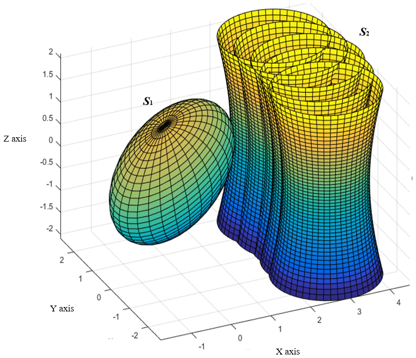
This indicates that the center of the sphere is usually on the y axis, and it is independent of the other two variables x and z. The iterative process is shown in Fig. 7.

Figure 7 An iterative process diagram of the ball to the ellipsoid.

The conjugate of the surface shows that the two surfaces revolve around their axis; the rotation angles are φ₁ and φ₂. When φ₁ is a constant, there must be φ₂ to make the two surfaces in contact in a conjugate form. The rotation surface S₂ should rotate at an angle to make the conjugate surface contact. The two rotating surfaces are very close when in contact, and their radius of rotation is very large, so the rotational motion of S₂ can be simplified as a translation. Assume that the unit vector of the translation direction is

$$\begin{array}{}\text{(39)}& \mathit{\delta }p=\left[\begin{array}{ccc}\mathit{\delta }{p}_x& \mathit{\delta }{p}_y& \mathit{\delta }{p}_z\end{array}\right],\end{array}$$

where δp_x, δp_y, and δp_z are only related to φ₂. Generally, the direction of translation is not along the shortest path between the two ellipsoids, but with an angle. Therefore, the distance along the translation path to the ellipsoid S₂ can be simplified as the projection of the shortest distance in the translation direction. Therefore, the approximate distance l can be expressed as

$$\begin{array}{}\text{(40)}& l=\mathit{\delta }p\left(r_{\mathrm{1}}-r_{\mathrm{2}}\right).\end{array}$$

When l is positive, it moves forward. On the contrary, when l is negative, it moves in the opposite direction. Figure 8 shows the process of the ellipsoid S₂ approaching S₁, which is an iterative process. When the direction δp of the shift is the same as the direction of the shortest distance, the root of the equation can be solved step by step. Conversely, when the angle between the two surfaces becomes larger, the impact of the ellipsoid curvature on the approximation process will be lower.

Figure 8 The solving process of the ellipsoid S₁ to the ellipsoid S₂.

Apply the above analysis method to analyze the tooth contact of the gear pair. First, the main curvature and main direction of the tooth surface are calculated. Then, the regional structure of the initial calculation point is simplified to the ellipsoid based on the simplifying principle. ECA is applied to a series of conjugate contact points on the tooth surface, and the meshing line is available. Finally, the relative main direction and the main curvature can be calculated according to the curvature characteristics of the two surfaces. The size and direction of the meshing point can also be calculated.

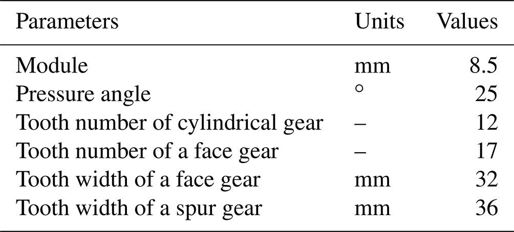
Taking the parameters shown in Table 1 as an example, the calculated contact cloud diagram of the face gear tooth surface is shown in Fig. 9. The tooth surface contact path of the front gear can be seen from the figure. To avoid excessive tooth-bottom undercut and tooth-top sharpening, the face gear width is designed to be 32 mm under the conditions of processing. The surface contact trace of the face gear is directed from the outer tooth top to the inner tooth bottom, which can meet the requirements of face gear transmission meshing contact. From the above analysis, it can be seen that the application of ellipsoidal surface contact analysis theory can quickly determine the meshing characteristics of the face gear tooth surface and effectively shorten the development cycle of the face gear.

Table 1 Face gear pair design parameters.

Figure 9 Contact-type cloud picture on the tooth surface.

6 Conclusions

This paper presents an ellipsoidal contact analysis method for the meshing tooth surface of a face gear. Ellipsoidal substituting of the meshing surface can simplify the choke contact process and avoid the singularity entering the analysis area, thus improving the iteration speed and stability. The numerical engagement method of the ellipsoid arc of high-order face gears can be extended to the contact process analysis of other complex surfaces. It provides a theoretical basis for the rapid integrated optimization design of face gears. Some conclusions are given as follows.

• 1.

  According to the characteristics of the face gear, the preferred method of the face gear flank sample point is established, the flank sampling point is meshed by three B-spline functions, the face gear flank fitting equation is derived, and a mathematical model is formulated to solve the contact point of the fitted flank using the composite method.

• 2.

  With the two-curve direction as the reference direction, the curvature of the surface at the determining point and the short-range deflection rate are obtained.

• 3.

  To simplify the solution of the conjugate motion relationship in the theory of flank conjugate, it is proposed to replace the conjugate surface with an elliptic body to simplify the digital iterative process into an analytical solution.