Influence of a walking mechanism on the hydrodynamic performance of a high-speed wheeled amphibious vehicle

In order to reduce the resistance and increase speed for a high-speed wheeled amphibious vehicle, a wheel-retracting mechanism was applied to a walking mechanism and the influence was researched. Firstly, to obtain a reliable numerical method, a realizable shear stress transport (SST) k-ω turbulence model and computational fluid dynamic (CFD) model built by an overset mesh technique was used and compared with the corresponding model tests. Secondly, the effect of the wheels' flip angle on resistance, heave and pitch was investigated. Then, the wheel well was optimized by numerical simulation. Finally, the results showed that the influence of the wheels on resistance was more significant, and the larger the wheels' flip angle was, the more significant the resistance reduction would be. An optimized wheel well was beneficial to resistance reduction. Furthermore, the running attitude became steadier, thereby decreasing the heave and pitch.

1 Introduction

A high-speed wheeled amphibious vehicle (HWAV) is one kind of amphibious vehicle. It is designed to carry out emergency rescues on the coast and meet the requirements of daily patrols and other tasks. The military and civilian markets favor the HWAV because of its high maneuverability on land, high-speed performance on water, and fast conversion performance on water and land. Among them, high-speed performance on water is the main performance of the amphibious vehicle, and it is also the performance index that scholars and experts engaged in the research of amphibious vehicles have focused on pursuing breakthroughs in recent years.

In researching the resistance performance of an HWAV, the numerical method can obtain detailed information by flow-field visualization and has obvious advantages in analyzing flow phenomena and resistance components compared to experiments. Wang (2020) investigated hydrodynamic performance of a double-carriage amphibious vehicle by towing tests and numerical simulation. And the numerically calculated result is essentially consistent with the total resistance of the model towing tank test. The research results showed that the hydrodynamic performance of the three-dimensional vehicle could be numerically predicted based on the realizable k-ε turbulence model and multibody overlapping grid technology (Wang et al., 2020). The resistance and stability of the wheeled amphibious vehicle were investigated by experimental model tests and computational fluid dynamic (CFD) analysis (More et al., 2014). High-accuracy hydrodynamic evaluation of the planned hull using CFD technology was studied (Sukas et al., 2017). The resistance of a multipurpose amphibious vehicle was studied using CFD techniques with Reynolds-averaged Navier–Stokes (RANS) model, which gives the viscous flow field around the hull (Nakisa et al., 2014). The CFD software STAR-CCM+ was used for the resistance prediction of an armored personnel carrier (APC) called BTR-80 (Islam et al., 2018). Numerical simulation based on the RANS volume of fluid (VOF) solver was conducted to investigate the hydrodynamic performance of a planing craft and the effect of a fixed hydrofoil on its wave resistance, and the reliability of the method was verified (Bi et al., 2019). Vehicle resistance and sailing attitude after wheel retraction were predicted by numerical simulation, and the resistance reduction effect after wheel retraction was analyzed (Zheng et al., 2015). Feng et al. (2022) designed a deformable track wheel in order to study the resistance characteristics of amphibious vehicles in the transition phase. And the numerical calculation method based on the RANS solver and the towing test method is used to analyze the hydrodynamic performance of the amphibious vehicle (Feng et al., 2022). To tackle threats arising from environmental change, developing wheeled armored vehicles with amphibious functions will inevitably become a trend in the future. The results of the simulation obtained through these two modes have been discussed and compared to develop an efficient tool for performing hydrodynamic performance analysis of amphibious-wheeled armored vehicles (Jang et al., 2019).

Figure 1 HWAV scaled-down printing model.

There is no special theoretical solution strategy for water resistance of amphibious vehicles, and the numerical method of speedboats is generally used. However, compared with speedboats, the hull structure of amphibious vehicles is complex, and the turbulence around the vehicle is serious, so a high-precision theoretical solution is very difficult to achieve. The optimal design of hydrodynamic configurations based on the towing test method of the scaled-down model is difficult, and the complex geometric configuration of the amphibious vehicle increases the scale effect of the real vehicle resistance conversion, which leads to an increase in error. Therefore, it is important to carry out accurate numerical simulation studies to obtain the key parameters affecting the hydrodynamic performance of amphibious vehicles and to optimize the design of hydrodynamic configurations.

In order to shorten the design and analysis period, the CFD technique has been widely used in flow-field analysis. In this paper, an HWAV was designed and researched based on CFD technology (Demirel et al., 2014). The results were compared with the corresponding test results for verification. CFD had been applied to analyze the influence of the wheels' flip angle on the resistance performance, and the resistance reduction had been explained in terms of the change in the wake flow field of the HWAV. In the end, the wheel well was optimized based on our requirement for vehicle performance on land and water.

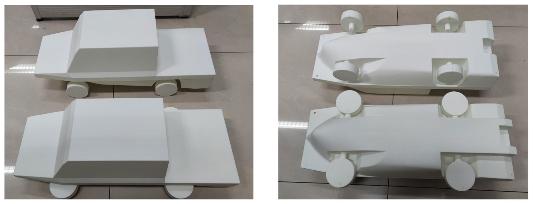
Three-dimensional printing technology was adopted to make the integrated HWAV model, designed with a ratio of 1:12 to the actual vehicle. As shown in Fig. 1, in order to explore the key factors to reduce resistance, in consideration of cost, time and accuracy, a CFD software package was utilized to conduct the simulation and then to provide a reference for subsequent model tests.

2 Numerical model

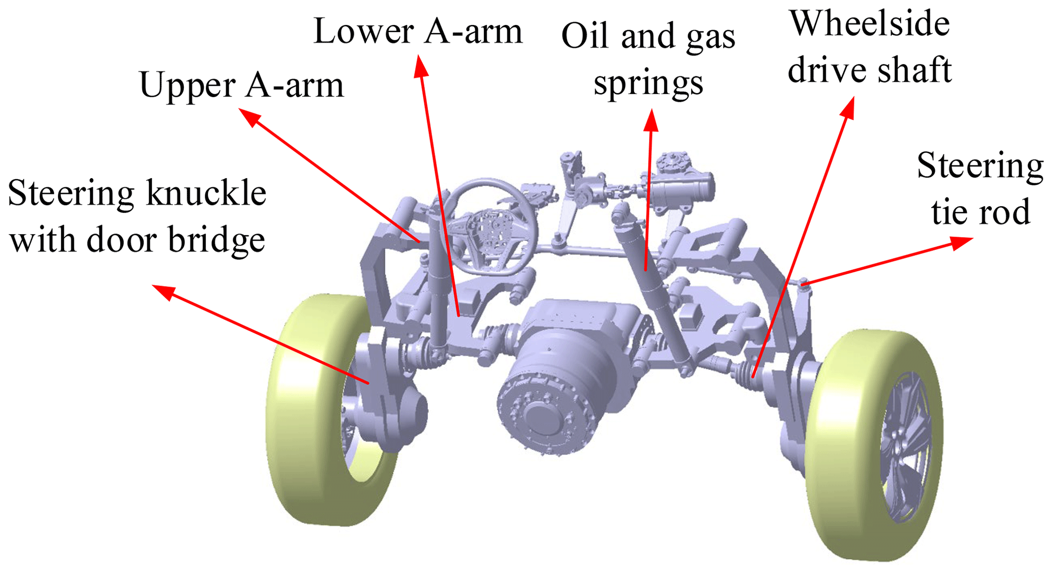
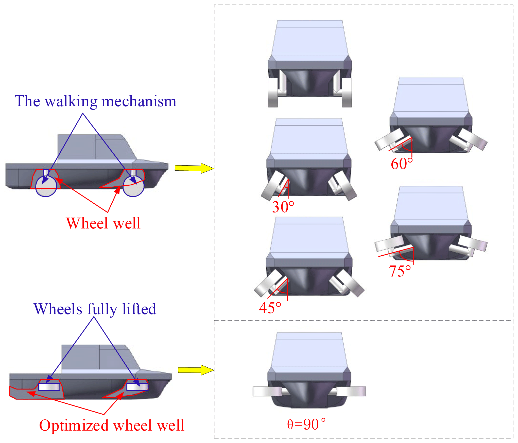
In response to the current amphibious vehicle water performance shortage, we innovatively designed the amphibious vehicle body and proposed a retractable mechanism applied to the walking mechanism. The HWAV studied in this paper adopted a deep V-shaped hull and wheel-retracting mechanism to reduce resistance, and the wheel-retracting mechanism adopts the shaped double A-arm portal suspension structure, as shown in Figs. 2 and 3. When moving on land, the oil and gas springs are equivalent to the use of conventional shock absorber assemblies, and the suspension system acts in the same way as the conventional suspension system to support the vehicle driving stability and damping; when sailing on water, the wheels are flipped as far as possible to reduce the resistance.

Figure 2 Double A-arm portal suspension.

Figure 3 Wheel flip status.

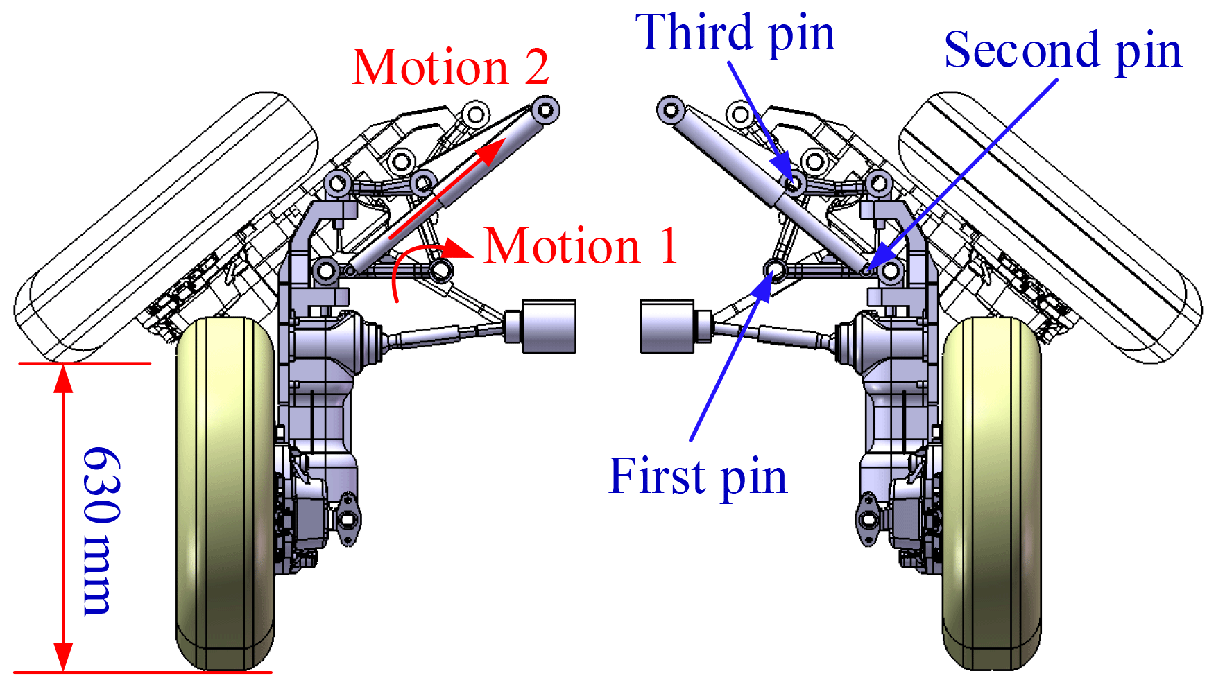
Compared to the traditional double A-arm suspension structure with a small buffering height of about ±100 mm, the retracting mechanism shown in Figs. 2 and 3 can lift the wheel to a large height of about 630 mm, by rearranging the positions of the pins on the hull, optimizing the lengths of the A-arms and especially by applying a door-bridge gearbox on the steering knuckle. Kinematics and dynamics analysis of the retracting mechanism showed that it is feasible for retracting the wheel out of water, and the retracting mechanism has enough strength to support the vehicle body while using titanium alloy materials. By controlling the length of the oil and gas spring, different flapping angles and heights of the wheel can be achieved.

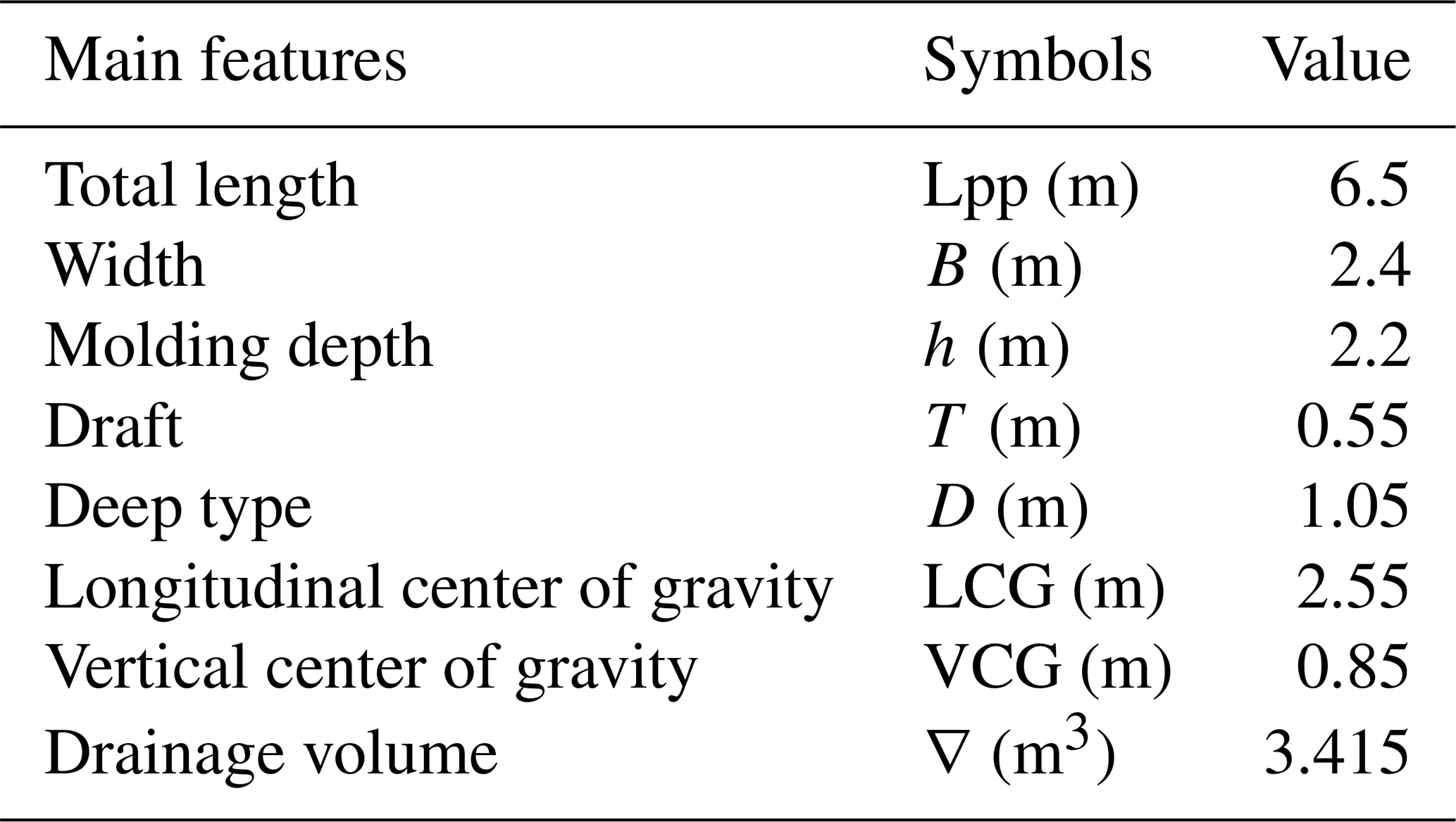
To facilitate the calculation, the hull model was simplified; the geometric design with different angles of wheel flip θ is shown in Fig. 4. The parameters of the simulation model are summarized in Table 1.

Table 1 Characteristics and coefficients of the HWAV.

Figure 4 Geometric model.

3 Numerical simulation approach

Although the amphibious vehicle is a type of equipment used both on the road and in the water, its hydrodynamic performance in water is similar to that of a conventional surface ship, and the numerical prediction of the relevant hydrodynamic performance based on computational fluid dynamic methods has been widely studied (Bi et al., 2019).

In this work, we focused on the HWAV. The flow field is simulated with a CFD solver package. The CFD solver has been successfully used to simulate the movement of the HWAV on water, and the accuracy of the solver has been validated extensively for flows with various amphibious vehicles and surface ships. It is worth noting that the present numerical simulation focuses on the fluid dynamics of amphibious vehicles sailing on water. It is not our intention to develop a numerical scheme.

Since the study in this paper involves the interaction between amphibious vehicle dynamics and fluid dynamics, the HWAV sail is in the horizontal plane, which is the same as our group's previous numerical simulations of amphibious vehicles (Sun et al., 2020, 2022). The above two verification cases are enough to show that our numerical method can accurately solve the hydrodynamic performance of amphibious vehicles.

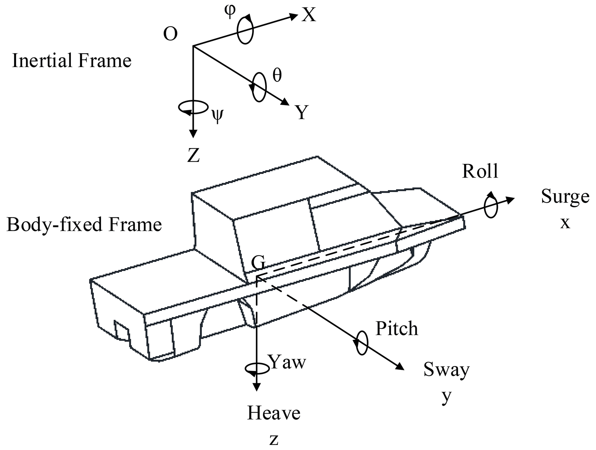
Describing the motion of the HWAV can be borrowed from the common ITTC (International Towing Tank Conference) coordinate system for ships, and two kinds of coordinate systems can be established, which are the fixed coordinate system and the motion of coordinate system. As shown in Fig. 5, the fixed coordinate system O–XYZ is one kind of inertial coordinate system. The motion of coordinate system G–xyz sets the origin G at the center of gravity of the hull. The motion coordinate system moves along with the hull and is mainly used to describe the rotational motion of the hull around the center of mass. At t=0, the origin of the spatial coordinates O coincides with the origin of the moving coordinate system G (ITTC, 2014).

Figure 5 The fixed coordinate system and moving coordinate system.

Figure 6 The dimensions of the calculation domains.

Figure 7 Boundary conditions.

3.1 Amphibious vehicle water motion equation

The motion of the HWAV satisfies the non-inertial rigid body momentum and momentum conservation equations, while the following assumptions are made for the model:

• (a)

  The moving coordinate system was fixed at the center of mass of the vehicle.
  

• (b)

  The vehicle was regarded as a rigid body.

Combining this with the previous assumptions, we can obtain the kinetic equations in the moving coordinate system as follows:

$$\begin{array}{}\text{(1)}& {\displaystyle }\mathit{m}\dot{\mathit{U}}+\mathit{m}(\mathbf{\Omega }\times \mathit{U})=\underset{S}{\int }\mathit{\tau }\cdot \mathit{n}\mathrm{d}s+mg+T\text{(2)}& {\displaystyle }\mathit{J}\cdot \dot{\mathbf{\Omega }}+\mathbf{\Omega }\times (\mathit{J}\cdot \mathbf{\Omega })=\underset{S}{\int }\mathit{r}\times (\mathit{\tau }\cdot \mathit{n})\mathrm{d}s+\mathit{R}\times T,\end{array}$$

where m is the hull mass tensor, U is the hull velocity vector, Ω is the hull angular velocity vector, J is the hull inertia tensor, τ is the hull surface stress (including pressure and shear) tensor, n is the unit normal vector of the opposite element ds under the conjoined coordinate system, g is the acceleration of gravity, T is the thrust force, R is the vector diameter from the point of thrust to the origin, r is the vector diameter from the element ds to the origin under the conjoined coordinate system and S is the closed surface of the body surface.

Figure 8 Mesh of the overall computational domain and the hull.

Figure 9 Overset mesh working principle.

Figure 10 Overset cell status.

Figure 11 The prism-layer grid of the hull surface.

Figure 12 Wall Y⁺ distribution of the hull surface.

Figure 13 Different grid schemes.

Table 2 The mesh parameters and calculation results.

Displacement and its derivative in a fixed coordinate system can be converted by the following two equations:

$$\begin{array}{}\text{(3)}& \left[\begin{array}{l}X\\ Y\\ Z\end{array}\right]=\left[\begin{array}{l}\cos \mathit{\phi }\cos \mathit{\theta }\\ \cos \mathit{\psi }\sin \mathit{\theta }\sin \mathit{\phi }-\sin \mathit{\psi }\cos \mathit{\phi }\\ \cos \mathit{\psi }\sin \mathit{\theta }\cos \mathit{\phi }+\sin \mathit{\psi }\sin \mathit{\phi }\\ \sin \mathit{\psi }\cos \mathit{\theta }\\ \sin \mathit{\psi }\sin \mathit{\theta }\sin \mathit{\phi }+\cos \mathit{\psi }\cos \mathit{\phi }\\ \sin \mathit{\psi }\sin \mathit{\theta }\cos \mathit{\phi }-\cos \mathit{\psi }\sin \mathit{\phi }\\ -\sin \mathit{\theta }\cos \mathit{\theta }\sin \mathit{\phi }\\ \cos \mathit{\theta }\cos \mathit{\phi }\end{array}\right]\cdot \left[\begin{array}{l}x\\ y\\ z\end{array}\right]\end{array}$$

$$\begin{array}{}\text{(4)}& \left[\begin{array}{l}\dot{\mathit{\phi }}\\ \dot{\mathit{\theta }}\\ \dot{\mathit{\psi }}\end{array}\right]=\left[\begin{array}{lll}\mathrm{1}& \sin \mathit{\phi }\tan \mathit{\theta }& \cos \mathit{\phi }\tan \mathit{\theta }\\ \mathrm{0}& \cos \mathit{\phi }& -\sin \mathit{\phi }\\ \mathrm{0}& \sin \mathit{\phi }/\cos \mathit{\theta }& \cos \mathit{\phi }/\cos \mathit{\theta }\end{array}\right]\cdot \left[\begin{array}{l}\mathit{\alpha }\\ \mathit{\beta }\\ \mathit{\gamma }\end{array}\right].\end{array}$$

Equations (3) and (4) form the kinematic equations of the HWAV, where α, β and γ are the angular velocities of rotation in the x axis, y axis and z axis in the moving coordinate system.

Figure 14 Total resistance coefficient values of CFD.

Figure 15 Waveforms of different grids.

Figure 16 Diagram of traction device.

Figure 17 Waveform comparison of towing test and simulation.

3.2 Turbulence model

When the HWAV is in the planing regime, the flow field around the hull will be turbulent. Therefore, the most widely used Reynolds-averaged Navier–Stokes (RANS) method is used to solve the computational problem of turbulence. For viscous and incompressible flows, the continuity and momentum equations can be described (Li et al., 2021) as

$$\begin{array}{}\text{(5)}& {\displaystyle \frac{\partial \left(\mathit{\rho }{u}_i\right)}{\partial x_i}}=\mathrm{0}\end{array}$$

$$\begin{array}{}\text{(6)}& \begin{array}{rl}{\displaystyle \frac{\partial \left(\mathit{\rho }{u}_i\right)}{\partial t}}& +{\displaystyle \frac{\partial \left(\mathit{\rho }{u}_i{u}_j\right)}{\partial x_i}}=-{\displaystyle \frac{\partial \mathit{\rho }}{\partial x_i}}\\ & +{\displaystyle \frac{\partial }{\partial x_i}}\left(\mathit{\nu }{\displaystyle \frac{\partial u_i}{\partial x_i}}-\mathit{\rho }\stackrel{\mathrm{‾}}{u_i{}^{\prime }{u}_j{}^{\prime }}\right)+S_i,\end{array}\end{array}$$

where i and j=1, 2 and 3; ρ is the density of the fluid; ν is the kinematic viscosity coefficient; u_iu_j is the instantaneous velocity component; $u_i{}^{\prime }{u}_j{}^{\prime }$ is the fluctuating velocity component; $\stackrel{\mathrm{‾}}{u_i{}^{\prime }{u}_j{}^{\prime }}$ is the average velocity component; and S_i is the source term.

The problem of the HWAV is the high Reynolds number flow. In the calculation for resistance, the turbulence model generally uses the SST k−ω model (Sun et al., 2022). The SST k−ω model retains the standard k−ω model near the wall and applies the k−ε model away from the wall, which is a hybrid model widely used in engineering and is particularly suitable for simulating flows in the presence of inverse pressure gradients. The k−ω model can compensate for the shortcomings of the k−ε model, which does not take into account the effects of turbulent anisotropy and has an excellent performance in the calculation of strongly separated flows. k and ω equations can be described as

$$\begin{array}{}\text{(7)}& \mathit{\rho }{\displaystyle \frac{\partial \left(k{u}_i\right)}{\partial x_i}}={\displaystyle \frac{\partial }{\partial x_i}}\left({\mathrm{\Gamma }}_k{\displaystyle \frac{\partial k}{\partial x_i}}\right)+G_k-\mathit{\rho }\mathit{\epsilon }\end{array}$$

$$\begin{array}{}\text{(8)}& \begin{array}{rl}\mathit{\rho }{\displaystyle \frac{\partial \left(\mathit{\epsilon }{u}_i\right)}{\partial x_i}}& ={\displaystyle \frac{\partial }{\partial x_i}}\left({\mathrm{\Gamma }}_{\mathit{\omega }}{\displaystyle \frac{\partial \mathit{\epsilon }}{\partial x_i}}\right)+\mathit{\alpha }{\displaystyle \frac{\mathit{\omega }}{k}}{G}_k-\mathit{\rho }{\mathit{\beta }}_i{\mathit{\omega }}^{\mathrm{2}}\\ & +\mathrm{2}(\mathrm{1}-F_{\mathrm{1}})\mathit{\rho }{\mathit{\sigma }}_{\mathit{\omega }\mathrm{2}}{\displaystyle \frac{\mathrm{1}}{\mathit{\omega }}}{\displaystyle \frac{\partial k}{\partial x_i}}{\displaystyle \frac{\partial \mathit{\omega }}{\partial x_i}}\end{array},\end{array}$$

where ${\mathrm{\Gamma }}_k=\mathit{\mu }+\frac{{\mathit{\mu }}_t}{{\mathit{\sigma }}_k}{\mathrm{\Gamma }}_{\mathit{\omega }}$ = $\mathit{\mu }+\frac{{\mathit{\mu }}_t}{{\mathit{\sigma }}_{\mathit{\omega }}}{G}_k$ = $-\mathit{\rho }\cdot \stackrel{\mathrm{‾}}{u_i{}^{\prime }{u}_j{}^{\prime }}$ $\frac{\partial u_j}{\partial x_i}{\mathit{\mu }}_t$ = $\frac{{\mathit{\rho }}_{c_{\mathit{\mu }}}{k}^{\mathrm{2}}}{\mathit{\epsilon }}$, F₁ = $\tanh \mathit{\{}{\left(min\left[max\left[\frac{\sqrt{k}}{\mathrm{0.99}\mathit{\omega }y}\frac{\mathrm{500}\mathit{\mu }}{\mathit{\rho }{y}^{\mathrm{2}}\mathit{\omega }}\right],\frac{\mathrm{4}\mathit{\rho }{\mathit{\sigma }}_{\mathit{\omega }\mathrm{2}}k}{{\mathrm{CD}}_{k\mathit{\omega }}{y}^{\mathrm{2}}}\right]\right)}^{\mathrm{2}}{\mathrm{CD}}_{k\mathit{\omega }}$ = $max\left[\frac{\mathrm{2}\mathit{\rho }{\mathit{\sigma }}_{\mathit{\omega }\mathrm{2}}}{\mathit{\omega }}\frac{\partial k\partial \mathit{\omega }}{\partial x_j\partial x_j},{\mathrm{10}}^{-\mathrm{20}}\right]$ represents cross-diffusion in the k-ω model. The constants in the equation are derived from theoretical derivations $c_{\mathit{\mu }}=\mathrm{0.09},{\mathit{\sigma }}_k=\mathrm{1.176},{\mathit{\sigma }}_{\mathit{\omega }}=\mathrm{2.0},\mathit{\alpha }=\mathrm{0.52},{\mathit{\beta }}_i=\mathrm{0.072},{\mathit{\sigma }}_{k\mathrm{2}}=\mathrm{1.0}and{\mathit{\sigma }}_{\mathit{\omega }\mathrm{2}}=\mathrm{1.168}$.

Figure 18 Total resistance values from experimental tests and CFD.

Figure 19 Sinkage and trim changes with Fr from experimental tests and CFD.

Figure 20 Resistance variation with Froude number at different wheels' flip angles.

3.3 Overset mesh setup

Although a common CFD software package is used in this paper, the numerical calculation of mesh as a key factor affects the CFD calculation results. For different calculation models, the required best meshing strategy is different. In this paper, through the evolutionary characteristics of the flow field around the HWAV in the process of a model towed test, the meshing strategy applicable to the HWAV numerical calculation is carefully designed.

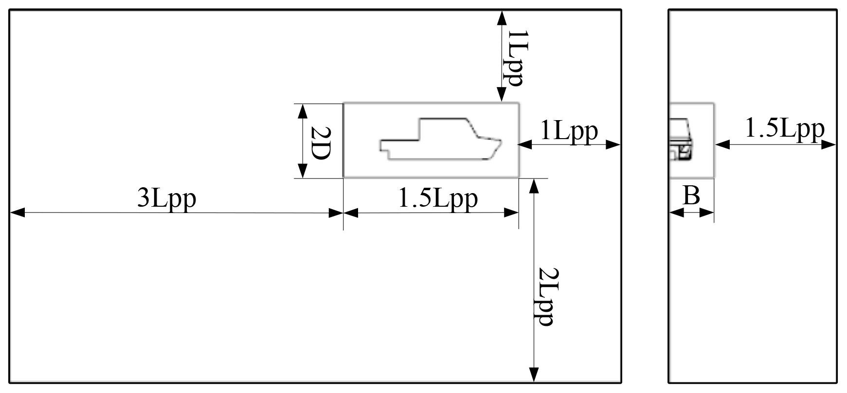
The size of the computational domain should be designed to ensure its reasonableness. A computational domain that is too small will affect the accuracy of the computational results, while one that is too large will lead to higher computational costs. According to the literature and guidelines given by the ITTC (Maki et al., 2016), selected dimensions of the calculation domains are as shown in Fig. 6.

Table 3 Parameters of towing test instruments.

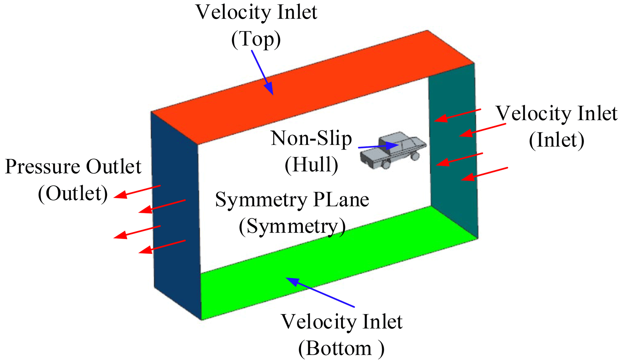
The boundary conditions were set as shown in Fig. 7. Considering that the simulation region is symmetric, only half of the model was calculated to save computational costs. The symmetry condition was applied to the symmetry plane and the side plane of the domain. The top and bottom was set as the velocity inlet, and all values were set equal to the hull speed. The outlet was defined as the pressure outlet, and the hull surface was set as the non-slip wall surface.

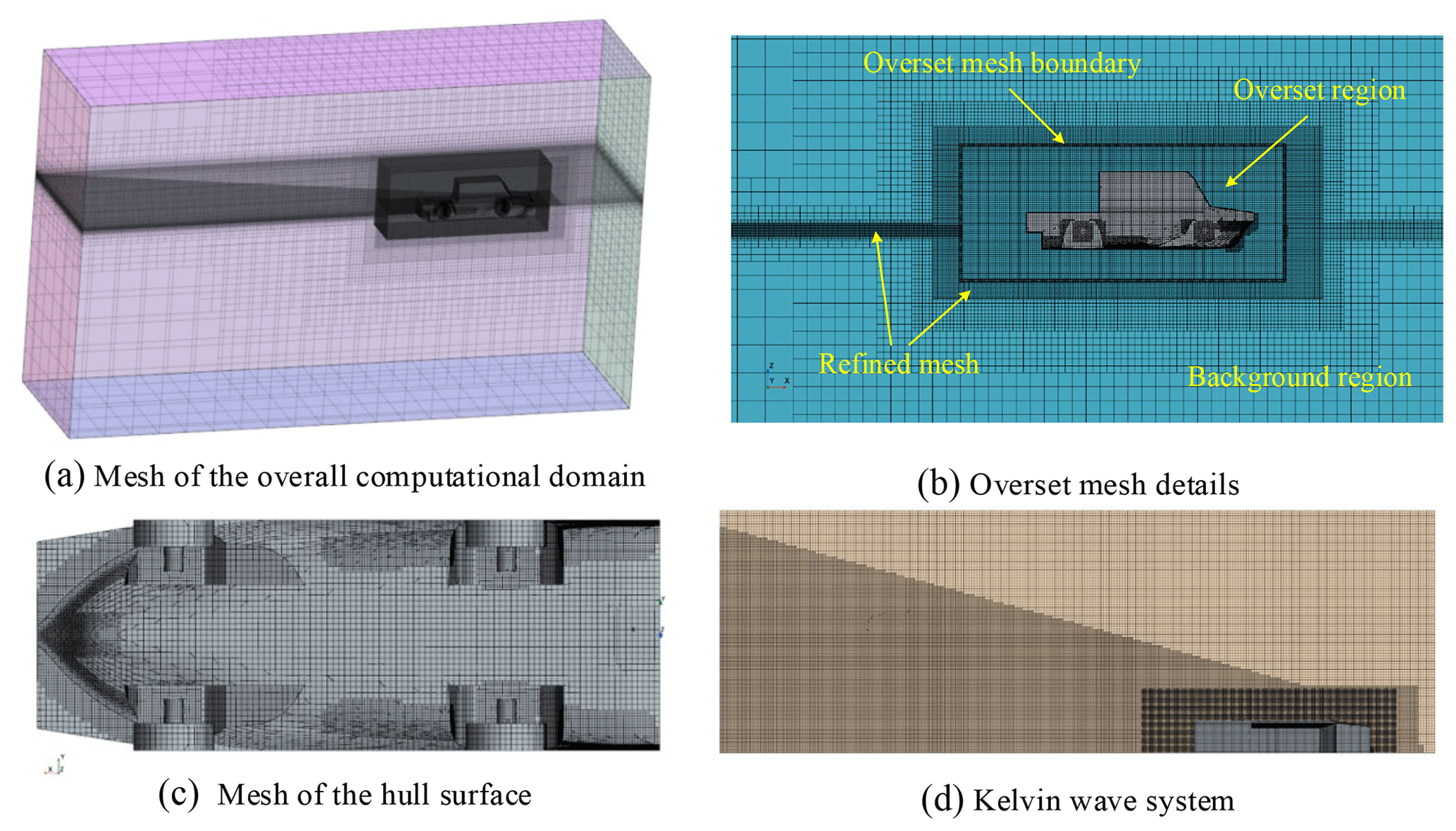
Mesh delineation is the key to the success of CFD simulation, and it directly affects the convergence and accuracy of the numerical results. The mesh quality will affect the convergence index and correction factor, which in turn affects the quantitative estimation of the time step uncertainty (Xing and Stern, 2010). In order to improve the computational accuracy, the flow fields around the hull and water surface were refined, and a Kelvin wave system was established, as shown in Fig. 8.

Table 4 Detailed results of resistance calculations.

The mesh generator of the CFD software package was used to generate the mesh of the computational domain, as shown in Fig. 8a. To solve the motion of the HWAV, two regions, the overset region and the background region, were used. As shown in Fig. 8b, the overset region moves together with the hull body. The background region is usually the computational domain adapted to the environment. Overlap boundary conditions were applied to the overset region embedded in the background region. The mesh generation was performed in the CFD software package. The software provides an overset mesh model that can accurately model large relative motions. In order to accurately calculate the flow field around the HWAV, the mesh around the vehicle was encrypted, as shown in Fig. 8c. The mesh encryption zone of the Kelvin wave system established based on the waveform caused by the HWAV observed in the towing test is shown in Fig. 8d.

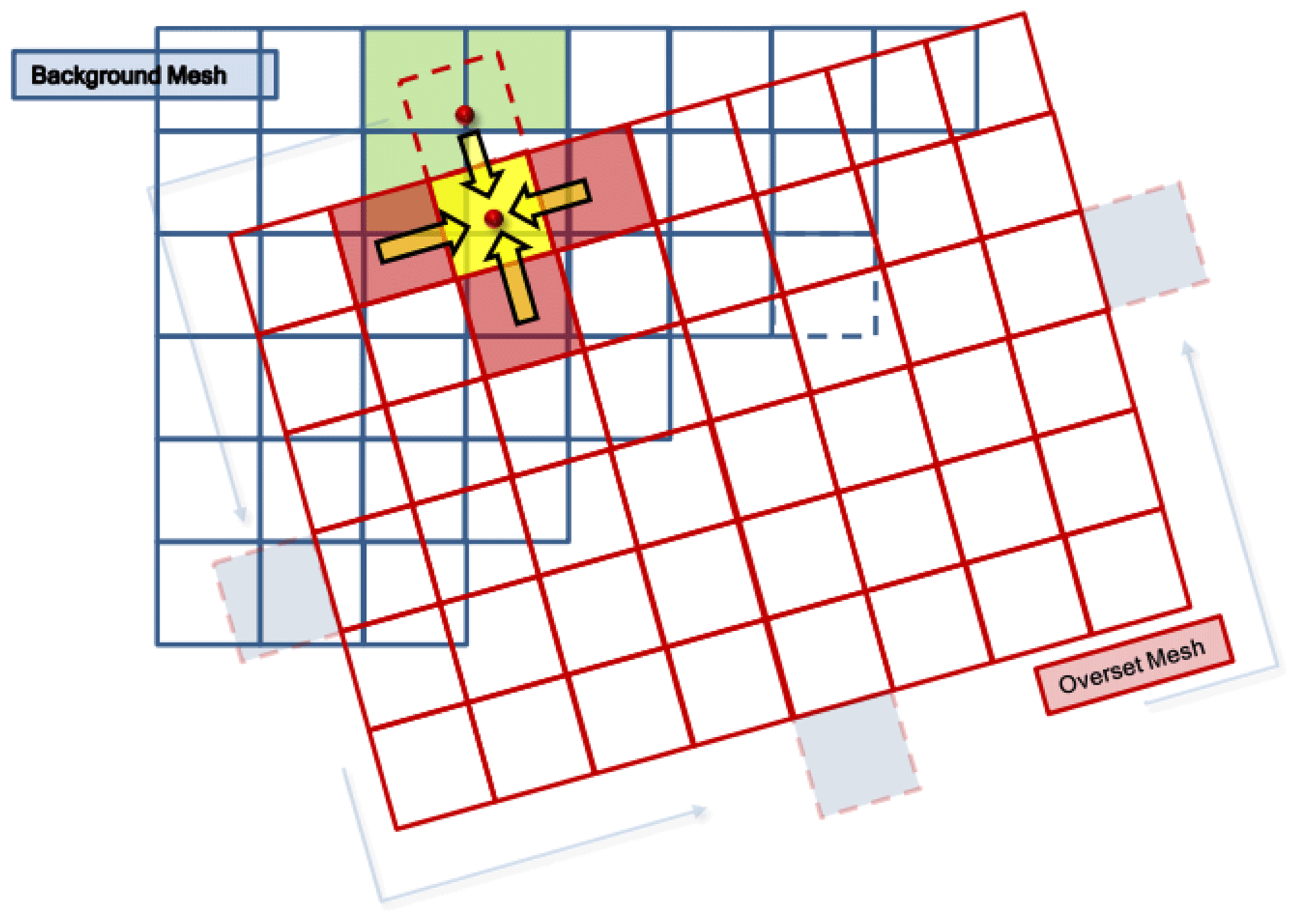
The working principle of the overset mesh system is shown in Fig. 9. Data are transferred from the overset mesh (red cells) to the background mesh (blue cells). The receptor cells (dashed lines) are used to provide information for the active cells (green and yellow).

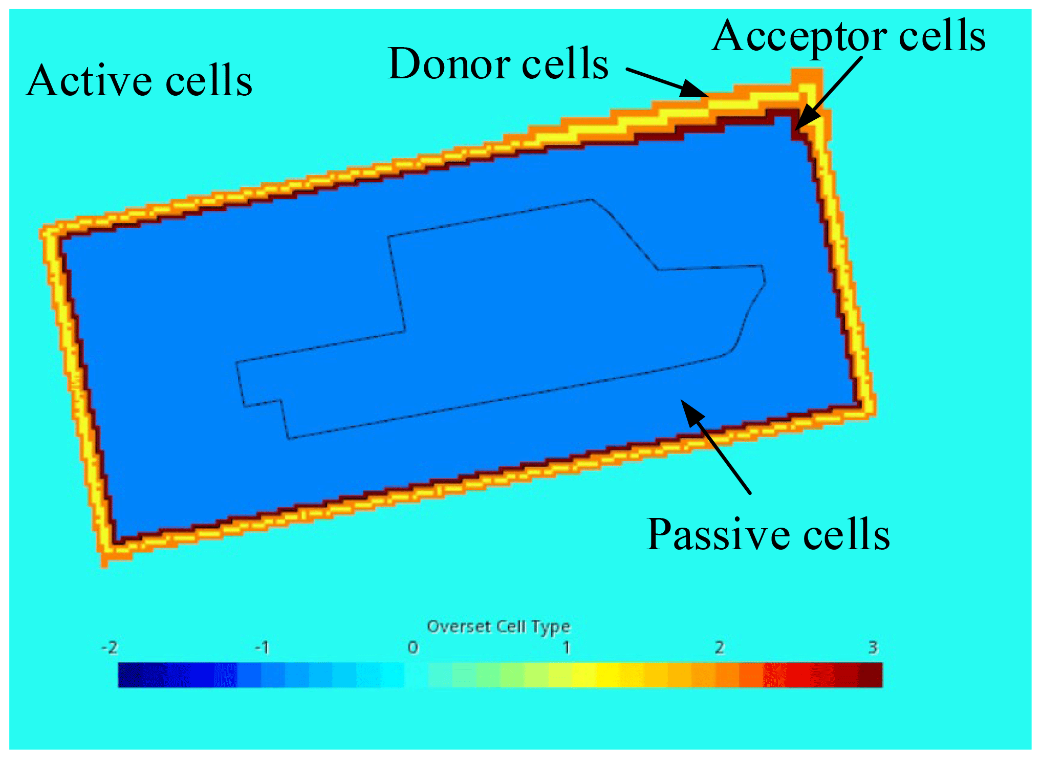
This method has four types of cells: the discredited control equations are solved in the active cell, the donor and acceptor cells provide and receive interpolation information respectively, the relationship between them is determined by the interpolation method, and the data interpolation occurs between grids, which can move with each other (Su et al., 2021). They are most useful in the simulation of multiple or moving objects and in parametric studies and optimization analysis. As shown in Fig. 10, their roles in the computation are as follows:

• active cells, where the discredited control equations are solved in these cells;

• donor cells, which provide interpolation information to the acceptor cells;

• acceptor cells, which receive information from the donor cells;

• passive cells, where no equations are solved.

The two meshes in the overlapping area should be the same size so that the data can be transferred linearly between them. Therefore, an overlapping interface is created between them, and the interpolation option is set to linear.

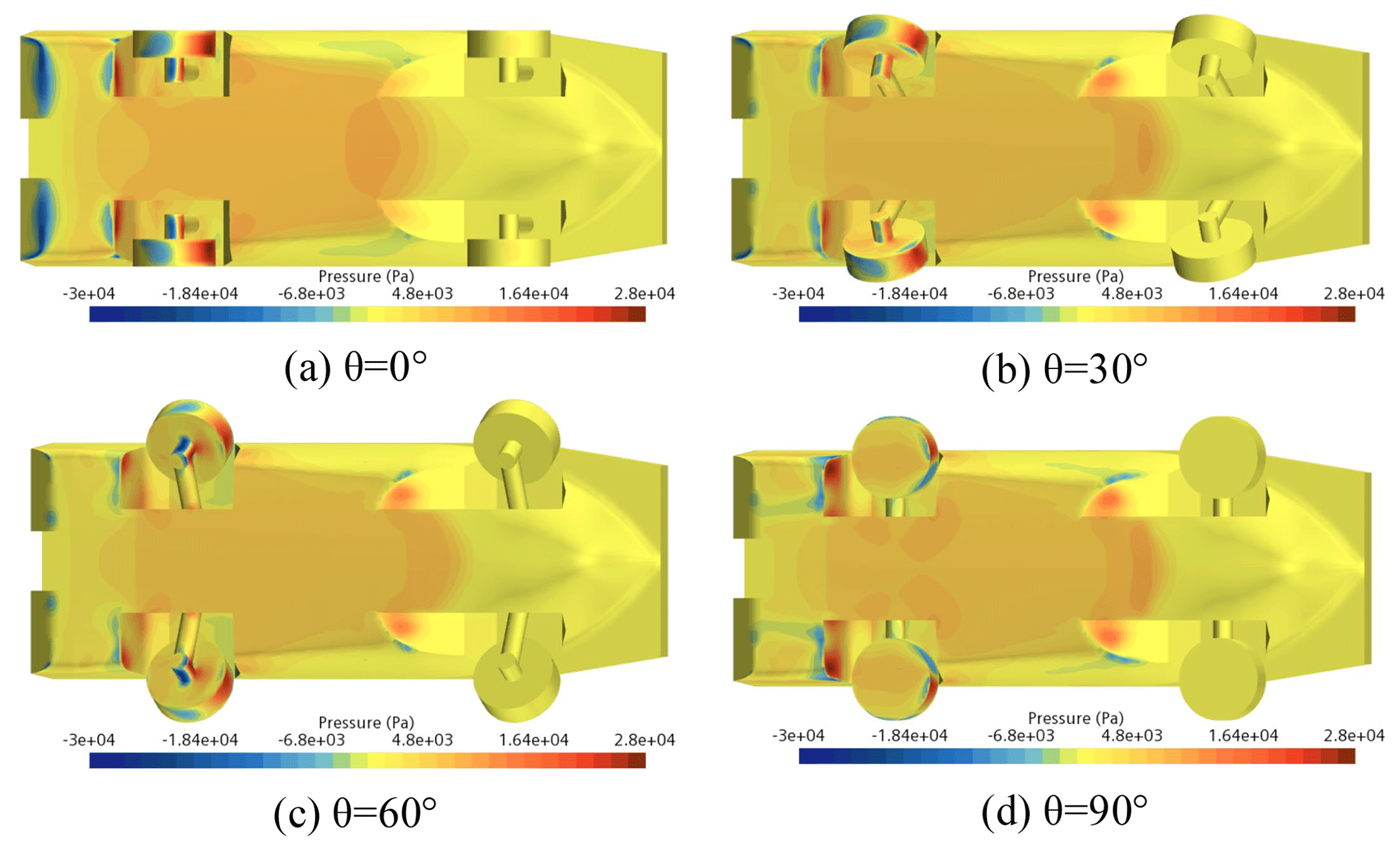
Figure 21 Pressure distribution on the hull surface with different wheels' flip angles at Fr = 0.87.

Figure 22 Water and gas two-phase diagram with different wheels' flip angles at Fr = 0.87.

3.4 VOF method and wall Y⁺

The problem of water surface motion refers to the dynamic simulation of the free surface, especially as when the motion of the HWAV generates complex wave-making, the free surface needs to be captured accurately. In this paper, the free surface between water and air had been tracked by the VOF model, which is commonly used in marine vehicles (Hirt and Nichols, 1981).

The basic principle of the VOF method is to calculate the volume ratio function P of the fluid in the grid cell. Here, the function P determines the boundary surface of the two-phase flow by realizing the volume change of the free surface (Scardovelli and Zaleski, 1999). The function P is defined as the ratio of the presence or absence of a specified fluid in the cell space to its occupancy. In brief,

• P=0: the fluid does not exist in the cell.

• $\mathrm{0}<P<\mathrm{1}$: an interface exists in the cell.

• P=1: the cell is filled with the specified fluid.

The function P satisfies the following differential equation:

$$\begin{array}{}\text{(9)}& {\displaystyle \frac{\partial P}{\partial t}}+u{\displaystyle \frac{\partial P}{\partial x}}+v{\displaystyle \frac{\partial P}{\partial y}}+w{\displaystyle \frac{\partial P}{\partial z}}=\mathrm{0}.\end{array}$$

In this study, dynamic fluid body interaction (DFBI) 6-degrees-of-freedom (6 DOF) models were used but only 2 DOF were required for simulating the real motion of the HWAV (Liang et al., 2019). Thus, except for the heave and pitch, the other 4 DOF were locked. To use this method, it is necessary to specify the relevant properties of the HWAV, including weight, the center of gravity and rotational inertia. In addition, to improve the accuracy and stability of the solution, the release time was set to make the fluid flow more uniformly, no translational or rotational motion occurs during this time and the ramp time was set to reduce the impact effect of the fluid on the hull at the beginning of the calculation (Song et al., 2020).

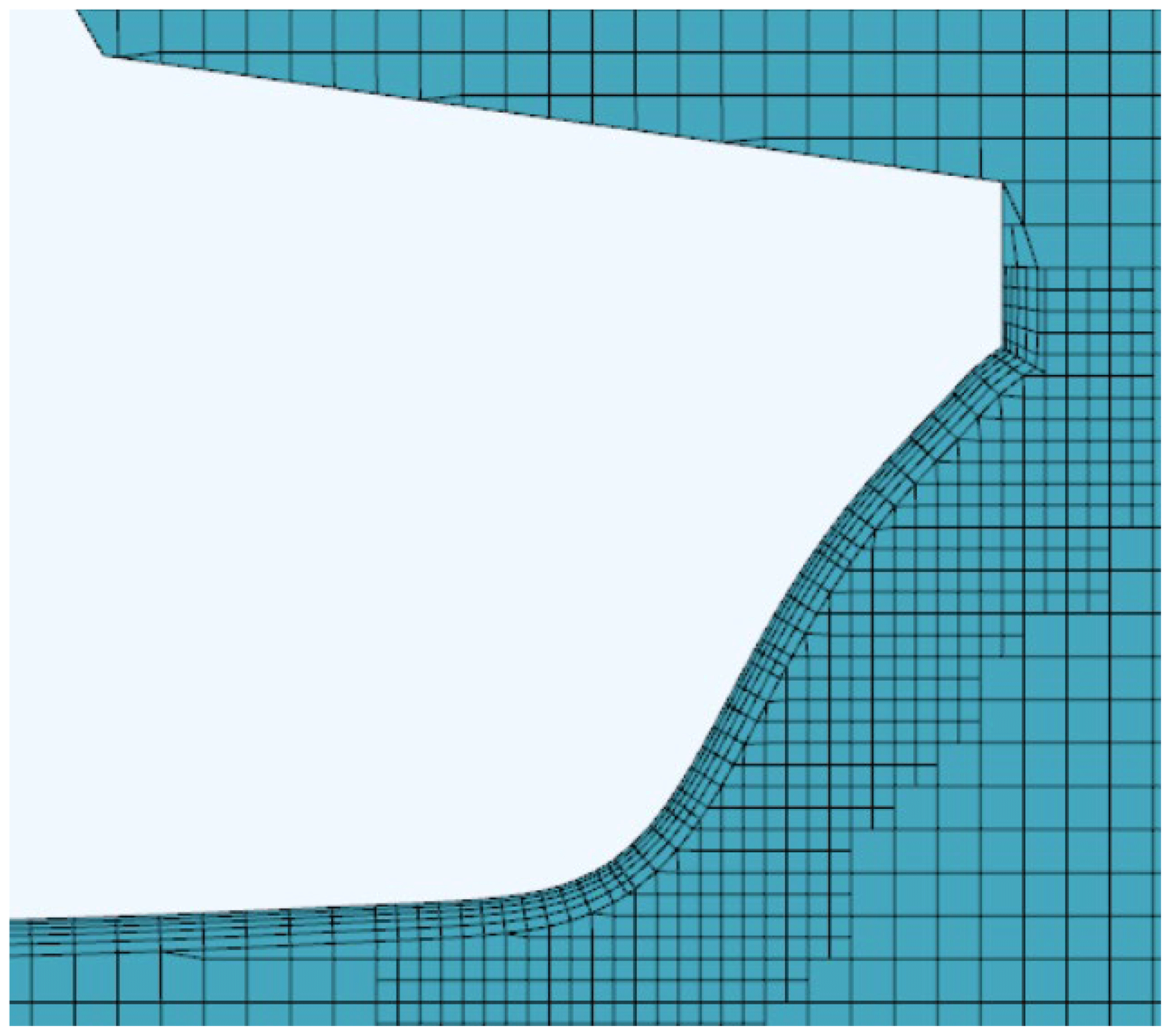
For turbulent numerical simulations, prism-layer grids are required, especially in cases of a high Reynolds number where the wall functions play an important role in the calculation accuracy. Figure 11 shows the prism-layer grids of the hull surface. Prism-layer grids were used on the hull surface to capture the boundary-layer flow and ensure that the grid's normal dimensions meet the requirements of the wall function application. The boundary-layer thickness can be calculated by the following equation:

$$\begin{array}{}\text{(10)}& {\displaystyle }\mathit{\delta }\left(x\right)=\mathrm{0.37}\times R{e}_x^{-\frac{\mathrm{1}}{\mathrm{5}}}\text{(11)}& {\displaystyle }R{e}_x={\displaystyle \frac{\mathit{\rho }{V}_{\mathrm{0}}{L}_{\mathrm{pp}}}{\mathit{\mu }}},\end{array}$$

where δ(x) is the boundary-layer thickness, Re_x is the Reynolds number, ρ is the water density at 20 ^∘C, V₀ is the vehicle speed and μ is the dynamic viscosity coefficient.

In classical fluid dynamics theory, prism-layer grids are used to generate boundary-layer grids, and the y⁺ value is the dimensionless distance from the wall to the first grid node. Currently, y⁺ is generally calculated using the following equation:

$$\begin{array}{}\text{(12)}& y^{+}={\displaystyle \frac{y}{\mathit{\upsilon }}}\sqrt{{\displaystyle \frac{\mathrm{1}}{\mathrm{2}}}{U}^{\mathrm{2}}{\displaystyle \frac{\mathrm{0.074}}{R{e}_L^{\mathrm{0.2}}}}},\end{array}$$

where y is the height from the first grid node of the boundary-layer grid to the wall, U is the speed of the HWAV, L is the waterline length of the hull and υ is the fluid viscosity coefficient.

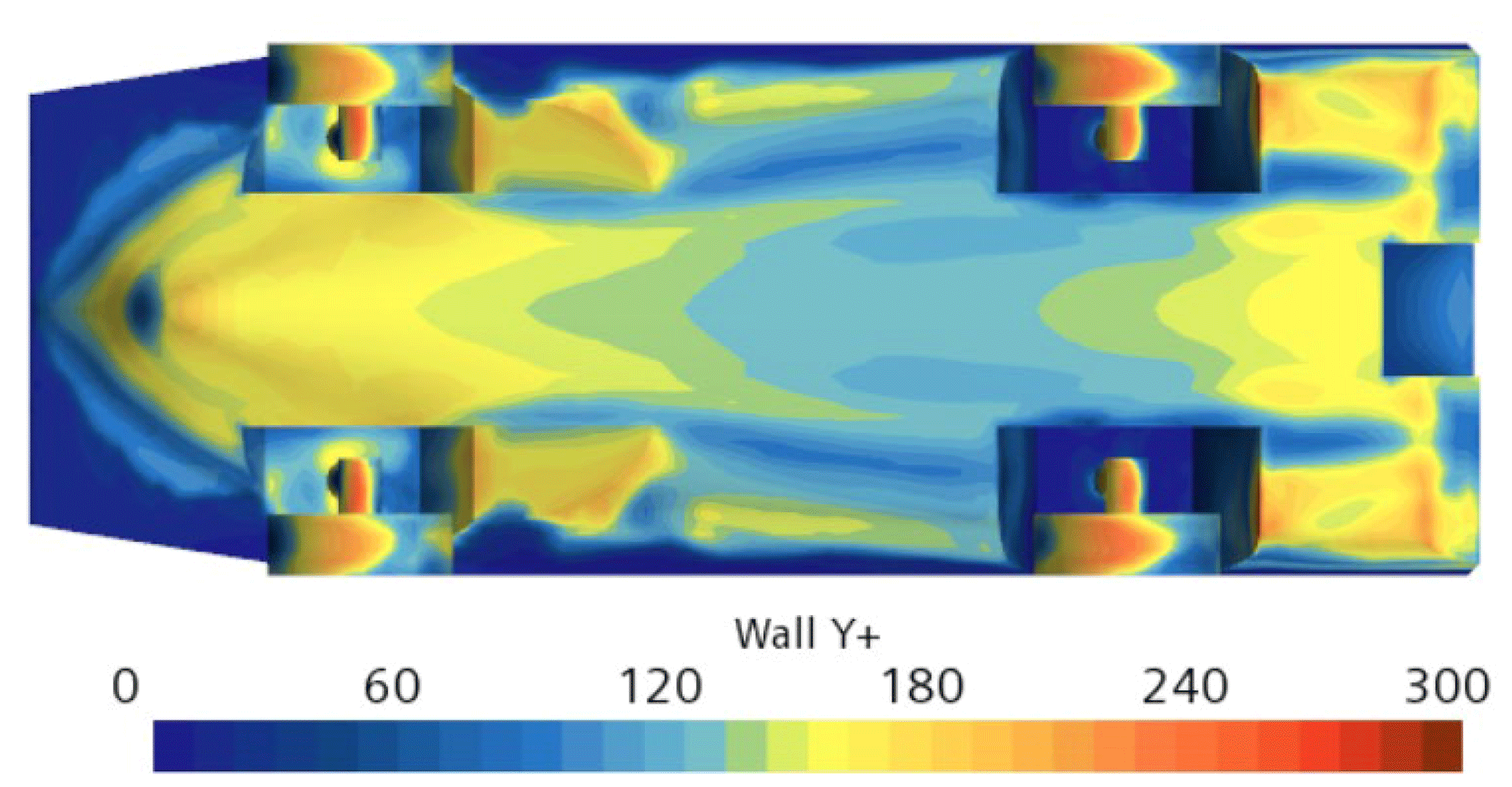
For general hydrodynamic calculations, the y⁺ value was controlled between 30 and 300, as shown in Fig. 12. For the model based on the wall function, five boundary layers with a grid growth rate of 1.1 were adopted.

3.5 Grid-independence verification

The use of a suitable number of meshes for calculation not only ensures the accuracy of the calculation results but also improves the calculation efficiency. For the uncertainty analysis of numerical calculation results, this paper developed three grid schemes for verification according to the CFD testing and the determined protocols recommended by ITTC (Zhu et al., 2007).

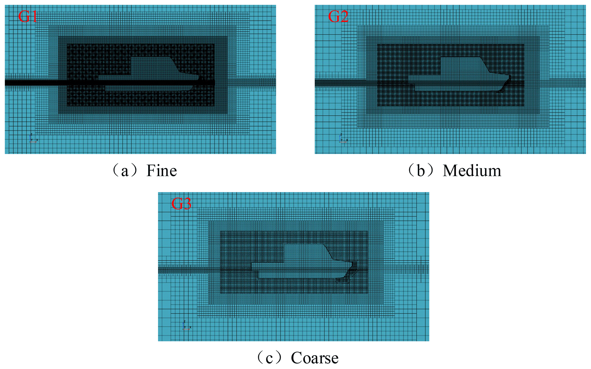
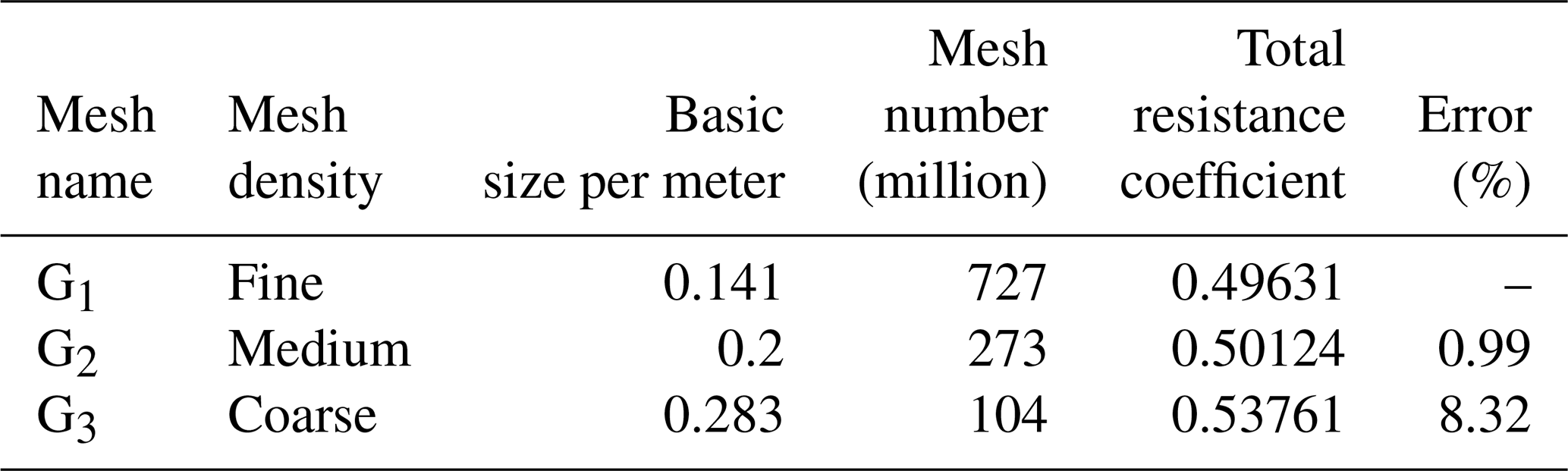
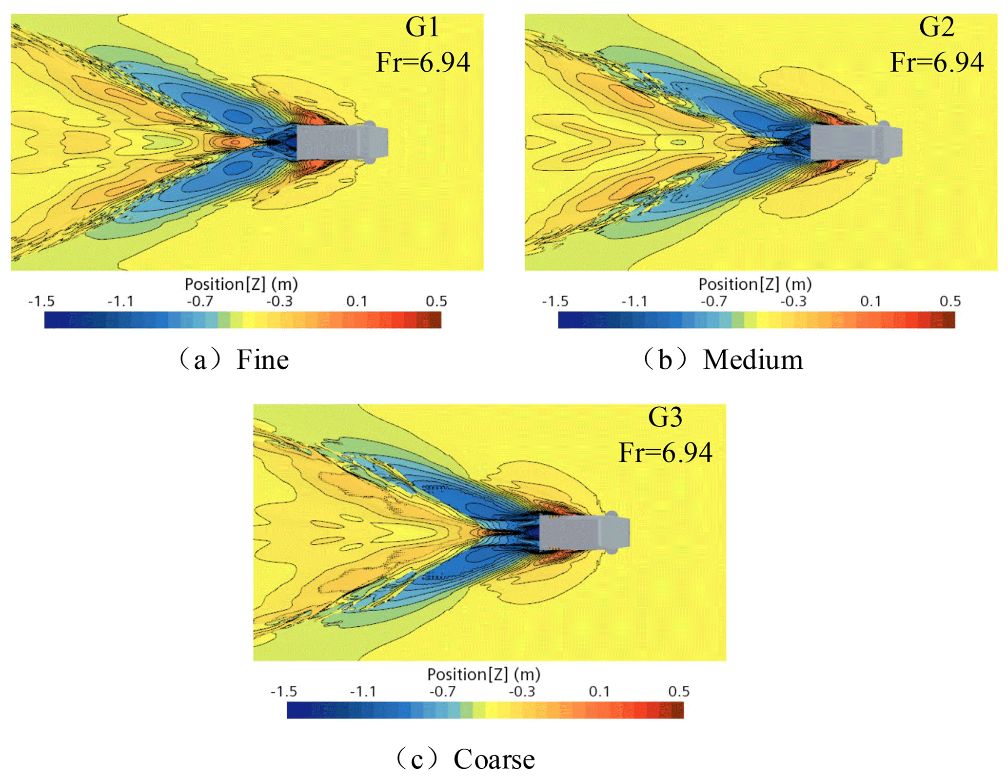
As shown in Fig. 13, the number of grids was adjusted by changing the value of the global grid's base size to ensure that the boundary-layer grids remained unchanged. The grid refinement ratio r_G was taken as $\sqrt{\mathrm{2}}$ (Momchil et al., 2019). The detailed parameters are listed in Table 2. The working conditions for validation are the Froude number as 0.87 and the time step as 0.02 s. As shown in Table 2, by taking the results of the fine grid model as the standard, the error of the results of the coarse grid and the medium grid was 0.99 % and 8.32 % respectively.

Figure 23 Sinkage and trim changes with Fr under various conditions.

Figure 24 Sinkage and trim at Fr = 0.696.

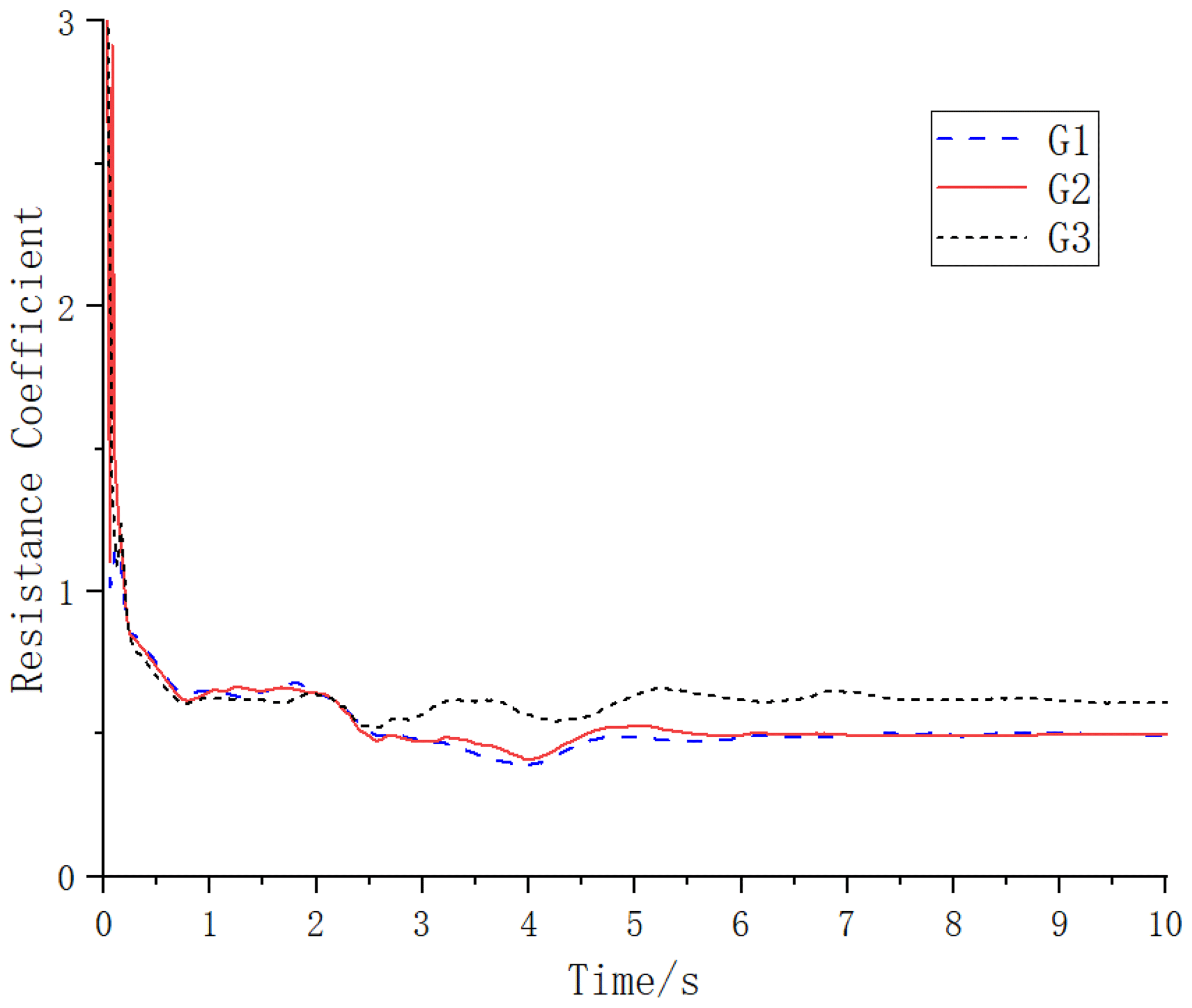
When comparing the total resistance coefficient of the three grid models, as shown in Fig. 14, the total resistance coefficient curves of the fine grid and the medium grid are almost the same (Fig. 15 shows the waveform plots of three different grids). It can be seen that the denser the grid is, the finer the waveform will be, where the waveforms of the fine and medium grids are almost the same, and the coarse grid has a larger error.

Three levels of the grid G₁, G₂ and G₃, respectively, correspond to the resistance values of $S_{G_{\mathrm{1}}}=\mathrm{7.671}$ kN, $S_{G_{\mathrm{2}}}=\mathrm{7.747}$ kN and $S_{G_{\mathrm{3}}}=\mathrm{8.448}$ kN, and the grid convergence ratio is calculated by $R_G=\left|\frac{S_{G_{\mathrm{1}}}-S_{G_{\mathrm{2}}}}{S_{G_{\mathrm{2}}}-S_{G_{\mathrm{3}}}}\right|=\mathrm{0.11}$, so $\mathrm{0}<R_G<\mathrm{1}$: the results meet the convergence requirements. Taking the computational accuracy and cost into consideration, the following simulations have been performed based on the mesh parameters of G₂ (Yanuar et al., 2017).

3.6 Numerical method validation

Based on the towing test of the HWAV, the numerical method in this paper was validated (Allaka and Groper, 2020). The towing resistance test was conducted in the towing pool of the Aviation Industry Corporation of the Chinese Academy of Special Aircraft Research, of 510.0 m (length) × 6.5 m (width) × 6.8 m (depth), with water depth and water temperature of 5.0 m and 25 ^∘C, respectively. A $\mathrm{1}/\mathrm{12}$ scaled model was manufactured, and the towing hull could operate in a stable speed range of 0.10–22.0 m s⁻¹, with a control accuracy of 0.2 %. The surface of the hull mold is waterproofed and painted to maintain smoothness and comply with the provisions of the allowable error standard. To obtain the sinkage and trim, 2 degrees of freedom (2 DOF) were released, that is, heave and pitch. A 10–15 min break was necessary between two consecutive tests to keep the water surface  calm.

Figure 25 Sinkage and trim at Fr = 0.87.

Figure 26 Sinkage and trim at Fr = 1.044.

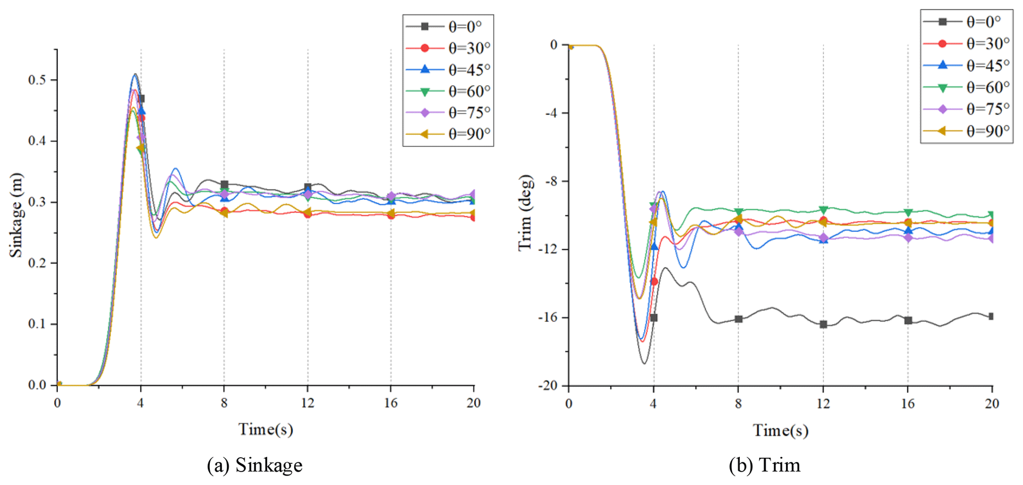
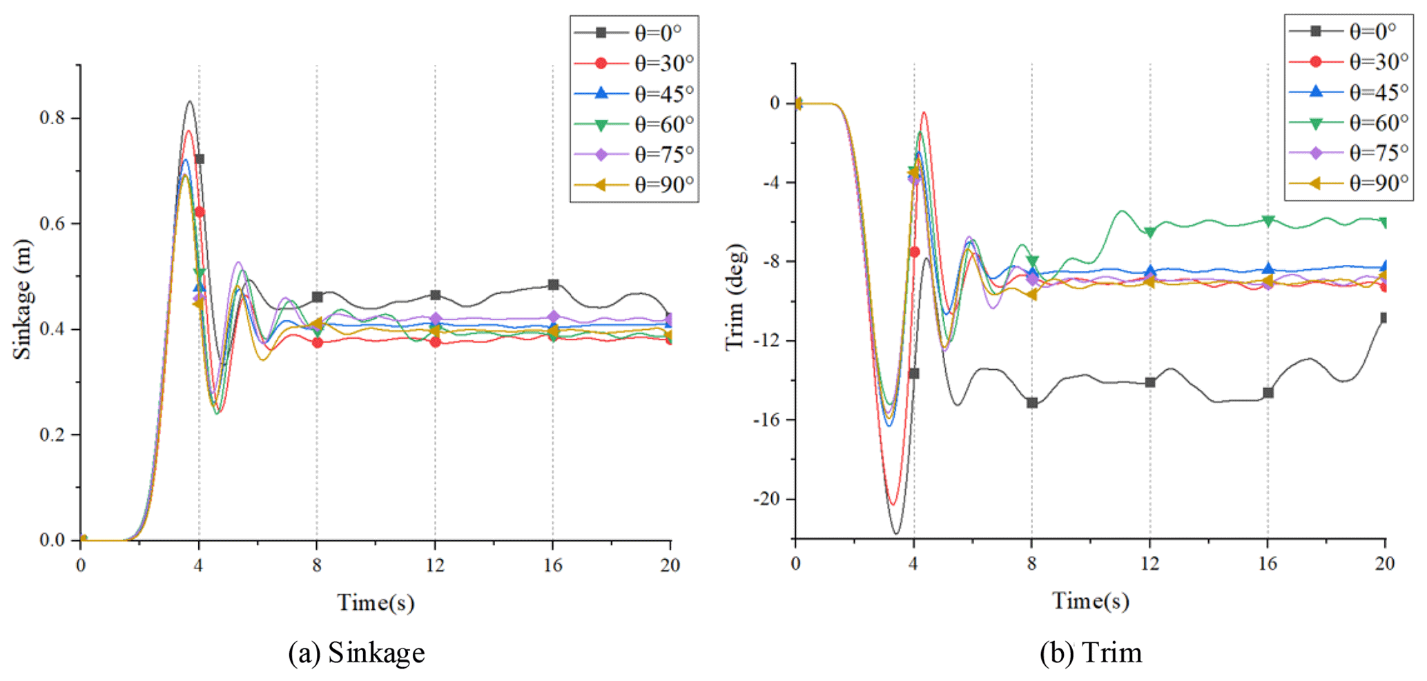
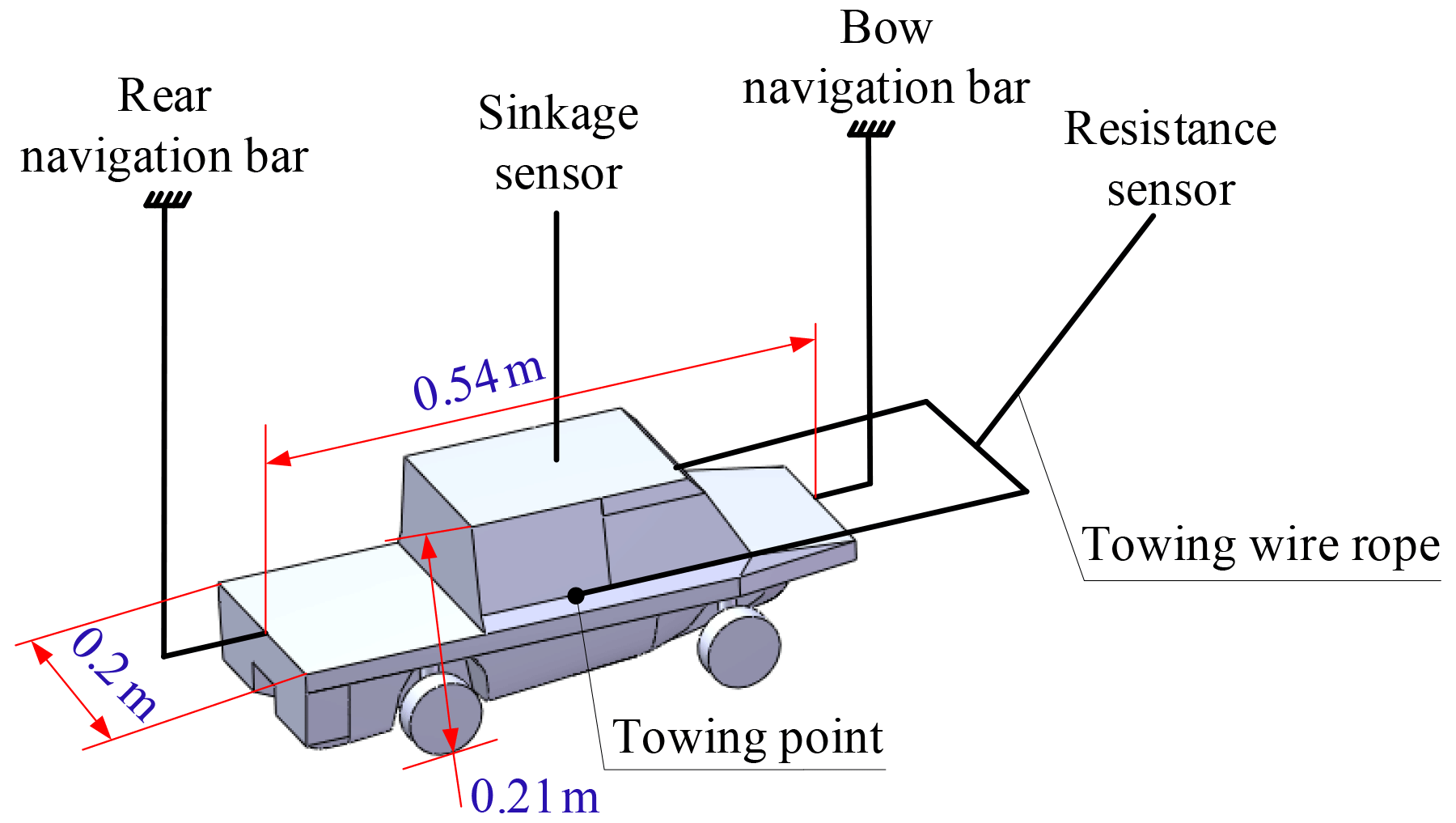
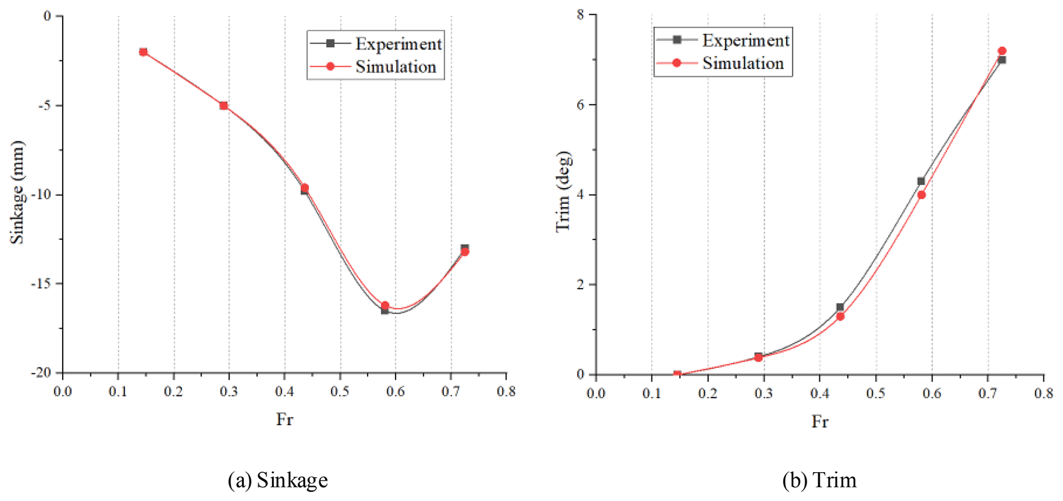
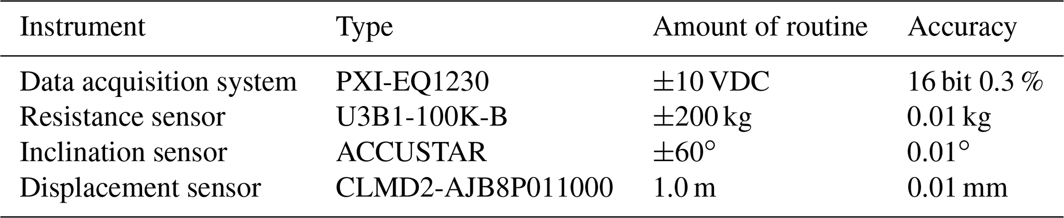
Figure 16 is a schematic diagram of the traction device. The resistance sensor is connected to the model towing point by a wire rope to ensure that the wire rope is located in the longitudinal plane of the model (Behara et al. 2020). The navigation bar is a vertical steel tube fixed to the trailer. The guide rail is mounted on the bow so that the navigation bar can pass through it. As the trailer moves forward, the hull is towed forward. At the same time, the hull can only heave (sinkage) and pitch (trim) under water pressure to measure sinkage and trim values (Ma et al., 2017). Trim and heave were free and could be measured by the inclination sensor and position sensor. The parameters of these instruments are given in Table 3 (Marquardt et al., 2014).

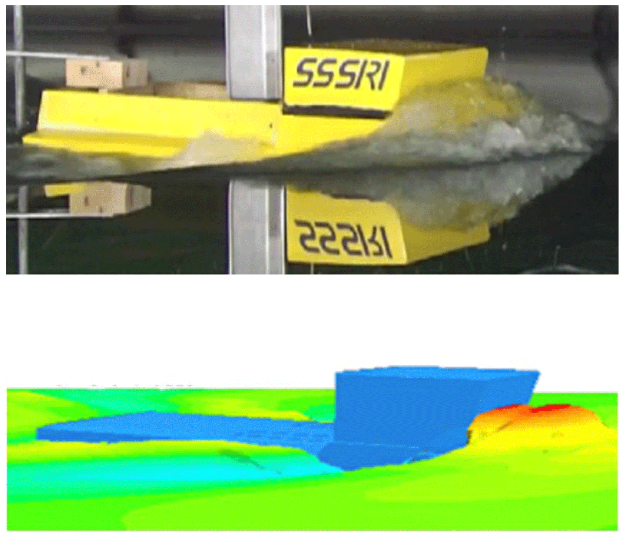
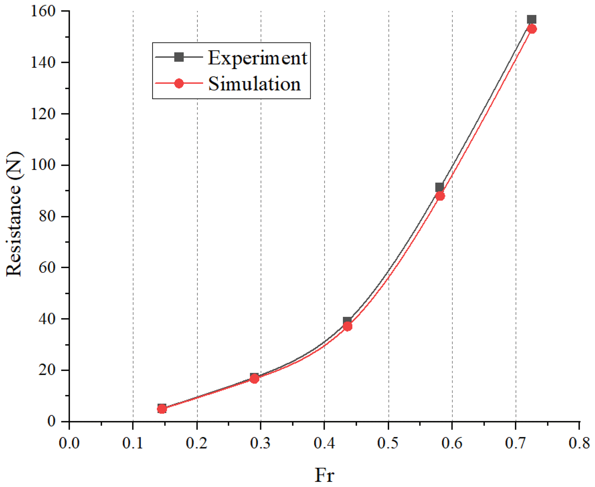
Figure 17 shows the experimental and simulation results of the hull at Fr = 0.436. It can be seen that the prediction of the navigation attitude of the hull can be effectively achieved using the simulation method, and the waveforms calculated by CFD are highly similar to the experimental results. The total resistance results of the experimental tests and numerical simulation are shown in Fig. 18. It can be seen that the resistance obtained by the test and CFD agree with an error of less than 8 %. This indicates that the method used in our research has high reliability. As shown in Fig. 19, results of sinkage and trim show good consistency, the average error is 6.16 %, and the maximum value error of 9.12 % occurs at Fr = 0.581. The sinkage and trim errors are more significant than resistance at high speed due to the large impact moment on the model caused by high-speed flow and the large trim angle, but the deviation was within the acceptable range.

4 Analysis of numerical results

The resistance of the HWAV at different Froude numbers and the resistance of the wheel flip at different angles were calculated, and the characteristic curves were plotted using simulation software.

The expression of the Froude number is as follows:

$$\begin{array}{}\text{(13)}& Fr={\displaystyle \frac{v}{\sqrt{g{L}_{\mathrm{WL}}}}},\end{array}$$

where v is the sailing speed of the HWAV, and L_WL is the length of the draft line.

Table 5 Sailing attitude at different wheel flip angles.

4.1 Influence of the wheel flip angle on hydrodynamic performance

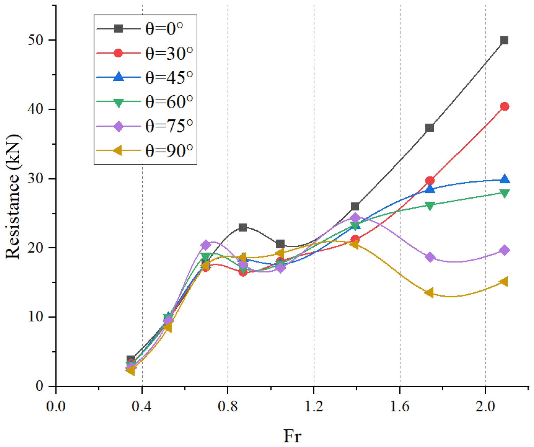
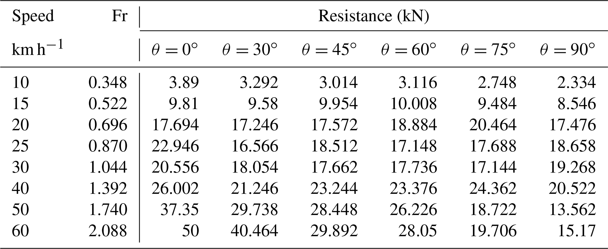
Table 4 shows detailed results of resistance calculations. With the increase of Froude numbers, the resistance of the vehicle increases at first and then decreases, and the peak of resistance appears between Fr = 0.696 and Fr = 0.87. The resistance peak is the threshold for the transition of the HWAV from the hull-borne to the planing regime. It requires the coordination of various measures such as resistance reduction and power increase to cross the peak. When the hull is in the planing regime, the resistance decreases rapidly, but the rate of decline decreases gradually. This is because, in the case of a low Froude number, the hull dynamic lift is small, and thus the wet area of the hull decreases slowly. According to Froude's assumption, the resistance is proportional to the square of the speed, so the resistance tends to increase with the increase of speed at this stage (Suneela et al., 2020).

Figure 27 Sinkage and trim at Fr = 1.392.

Figure 28 Comparison of resistance before and after the wheel-well optimization.

As Fig. 20 shows, in the low Froude number, the resistance is too small to get a significant resistance reduction effect. Therefore, the resistance reduction measures should be focused on the high Froude number. The peak of resistance can be reduced by retracting the wheels, and the best effect of resistance reduction occurs when the wheels are flipped at 30^∘, with a reduction of about 28 %.

When the hull was in the planing regime, the resistance reduction was more notable; that is, the resistance gradually decreases as the wheels' flip angle increases, and when the wheels flip to 90^∘, the resistance is reduced to the lowest. Because the wheels have been lifted, the smooth flow line of the hull bottom improves the flow state of water and reduces the vortex, which plays an important role in resistance reduction. The higher the Froude number is, the more significant the resistance reduction effect will be.

Figure 21 shows the contour of the hull pressure distribution with different wheels' flip angles at Fr = 0.87. With increasing the wheels' flip angle, the pressure decreases at the stern of the hull, and the pressure area on the wheels is significantly reduced. This could explain why the resistance is reduced by about 20 %–30 % at Fr = 0.87.

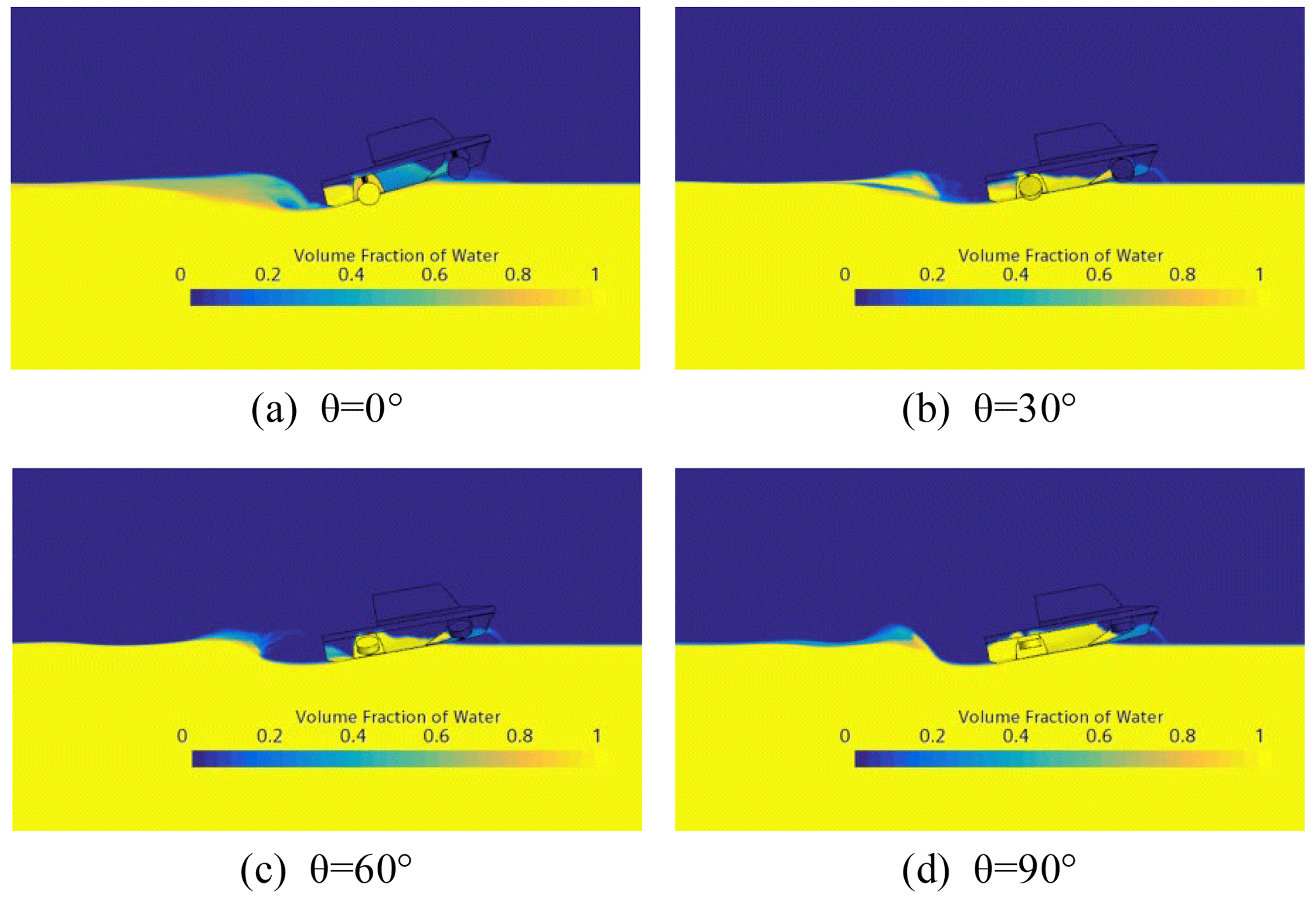
Figure 22 is the water and gas two-phase diagram of the hull with different wheels' flip angles at Fr = 0.87. It can be seen that the rear part of the hull produced a large water wave when the wheels are not flipped, and as the wheels' flip angle increases, the water line at the rear of the hull becomes longer and the transition is smoother without negative pressure. Moreover, at the rear part of the wheels not flipped, there is an obvious flow vortex, as shown in Fig. 22a; when the wheels are flipped, the water flow had good directionality, as shown in Fig. 22b–d.

Figure 29 Comparison of sinkage and trim before and after the wheel-well optimization.

When the wheels are not lifted, due to the attack angle of the protruding wheels, the water flow is affected in changing the stability of the flow and producing stagnation, so that a high-pressure area is formed at the front of the wheels' protrusion, and a low-pressure area appears at the rear of the wheels, and then negative pressure is generated. Vortex loss is generated and will increase the resistance; since the water velocity increases, the resistance increases further.

Figure 30 Water and gas two-phase diagram at Fr = 0.87.

Figure 31 Free wave surface at Fr = 0.87.

Figure 32 The rear wheel-well pressure diagram at Fr = 0.87.

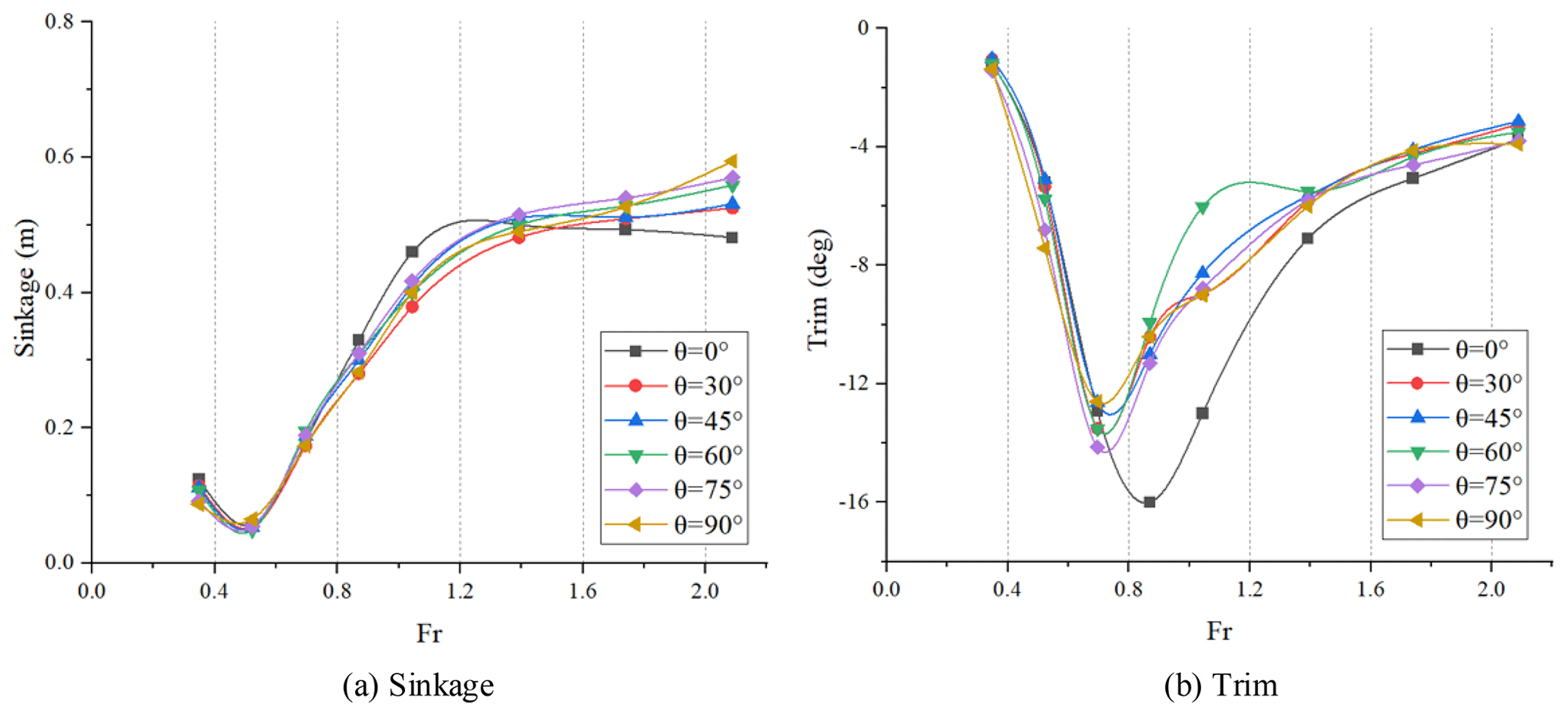
Heave and pitch will also affect the sailing resistance of the HWAV to a great extent. Increasing heave will reduce the wet area and then decrease its resistance. Increasing the pitch will increase the inflow angle and produce more violent waves. Figure 23 shows the sinkage and trim of the hull under different wheels' flip angles, and the sinkage and trim values correspond to the heave and pitch, respectively. The sinkage is defined as positive when the gravity center moves upward, and the trim is defined as positive when the hull bow rotates upward around y axis.

It can be inferred that the sinkage and trim firstly decrease and reach their minimum values, and then increase along with the enlargement of Froude number; this is because the increase of hull speed and the pitching moment cause the bow to rise and the stern to fall. When Fr<0.87, the wheels' flip angle has less effect on the sinkage and trim of the HWAV. When $\mathrm{0.87}<Fr<\mathrm{1.392}$, as the wheels' flip angle increases, the sinkage and trim gradually decrease, which makes the vehicle draft decrease, so flipping the wheels is beneficial to improve sailing attitude of the HWAV in this stage. And the hull can obtain the best heave and trim effect when Fr = 1.044 with θ=60^∘. When θ=30^∘, it can significantly reduce the sinkage of the vehicle during the planing regime, but it will increase the trim, making sailing the vehicle unstable. So the HWAV can improve the sailing attitude by adjusting the wheels' flip angle flexibly when sailing on water, which also provides a reference for subsequent research.

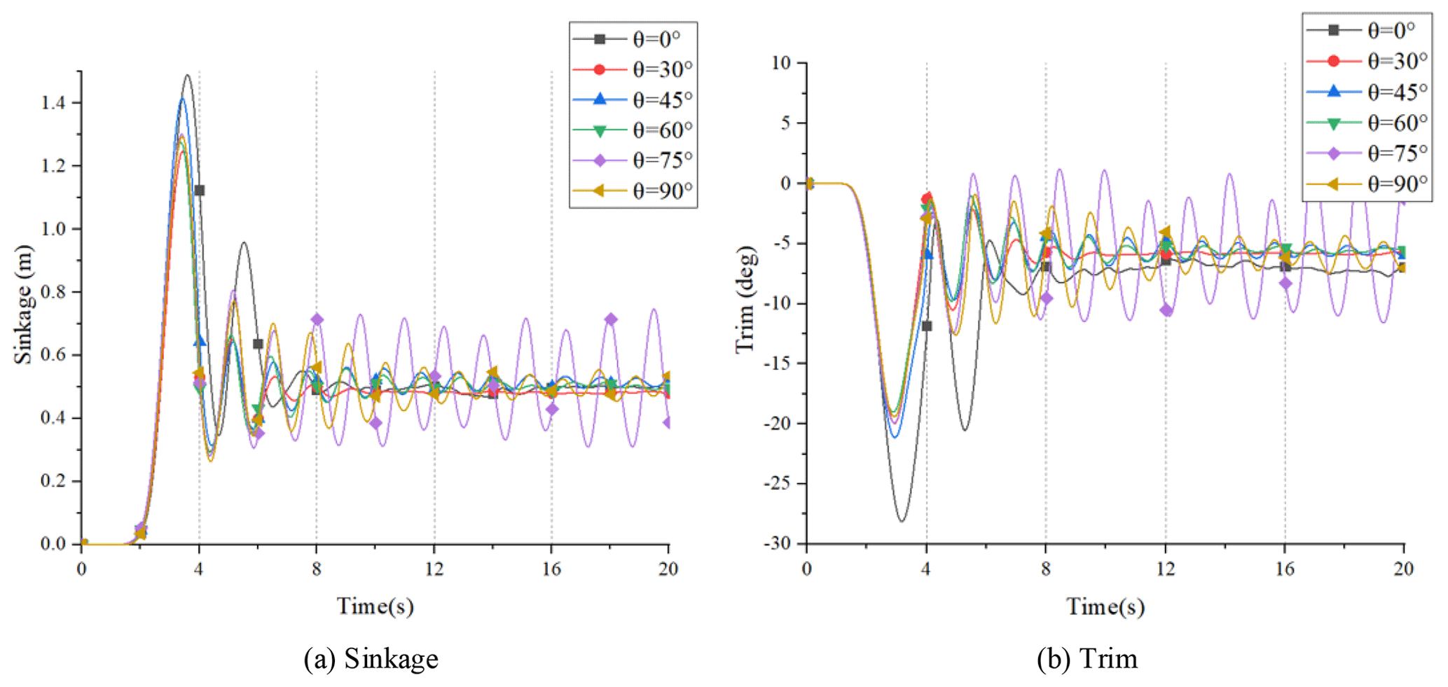
To more intuitively describe the sailing attitude of the HWAV at different wheels' flip angles, Figs. 24, 25, 26 and 27 give the conditions of the HWAV for four typical Fr values.

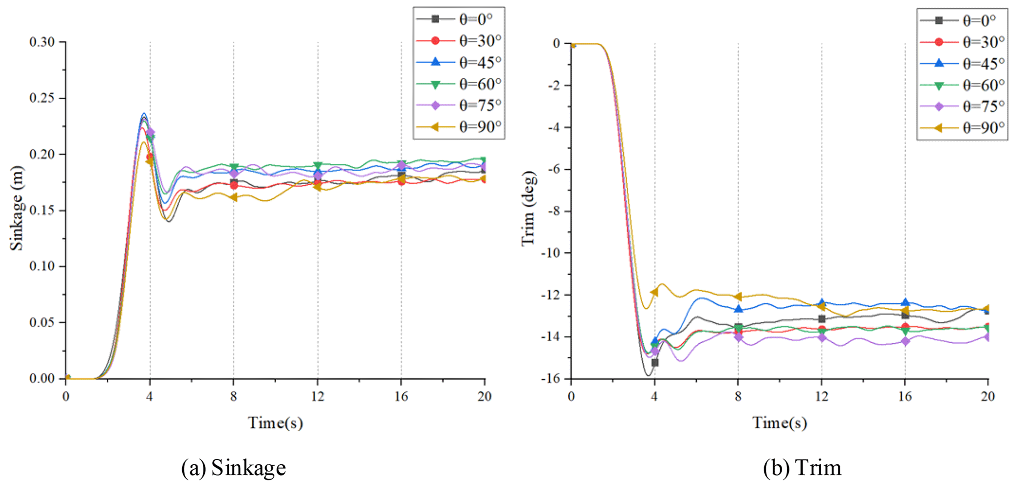
In Fig. 24, the vehicle showed only minor sinkage and trim motion fluctuations because of the low speed. In Figs. 25 and 26, under different wheels' flip angles, the sinkage and trim motion responses of the HWAV are much smaller compared to θ=0^∘. And when the wheels are not flipped, the sinkage and trim of the hull fluctuate greatly, making the movement of the hull unstable. Meanwhile, flipping wheels when the HWAV is in the planing regime can effectively reduce the amplitude of heave and pitch of the hull, and the effect on the pitch is more obvious. Therefore the amphibious vehicle can run more steadily. But in Fig. 27, it can be seen that the vehicle's motion responds with large fluctuations at high speed, especially when θ=75^∘. Therefore, when the HWAV is at a high speed, adjusting the wheels' flip angle reasonably can effectively improve its longitudinal stability.

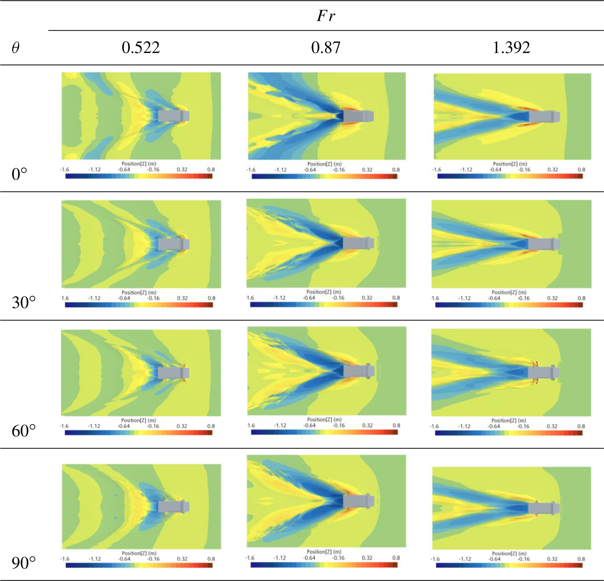
Table 5 shows the sailing attitude and waveform when Froude numbers are 0.522, 0.87 and 1.392. The diagram helps to better clarify the attitude change of the HWAV and the effect of the wheels' flip angle in the transition stage. When Fr = 0.522, the change of the wheels' flip angle has little influence on the sailing attitude. But when the Froude number is between 0.87 and 1.392, there is a significant change in the sailing attitude. When Fr = 0.87, the bow has left the water and the trim has reached the maximum, one of the reasons for the resistance peak. In this stage, flipping wheels can significantly reduce the trim of the hull. When Fr = 1.392, the sailing attitude begins to stabilize, and the vehicle gradually enters the planing regime.

This indicates that the wheels' flip angle affects the performance of the HWAV mainly at medium and high speeds. Wheels usually change the flow-field distribution around the hull, so it is important to study the change of the flow field to explain the mechanism of the wheels' influence on resistance performance.

4.2 Influence of the wheel well on hydrodynamic performance

For an HWAV, wheel-well design is important. The wheel well destroys the hull line, and the wheel well is in direct contact with the water surface, which will increase the resistance of the hull.

The design of the HWAV needs to consider the performance to move on land, so the hull is generally presented as a non-streamlined body. Since the curvature of the stern changes greatly, it has a greater impact on the hydrodynamic performance of the HWAV when sailing on the water. Vortex is often generated at abrupt changes of the hull curvature, especially at the stern. The closer to the center of the vortex, the lower the pressure will be, and then the vortex creates a suction force that hinders the hull's progress. In order to reduce the resistance, the design of the rear wheel well has been optimized.

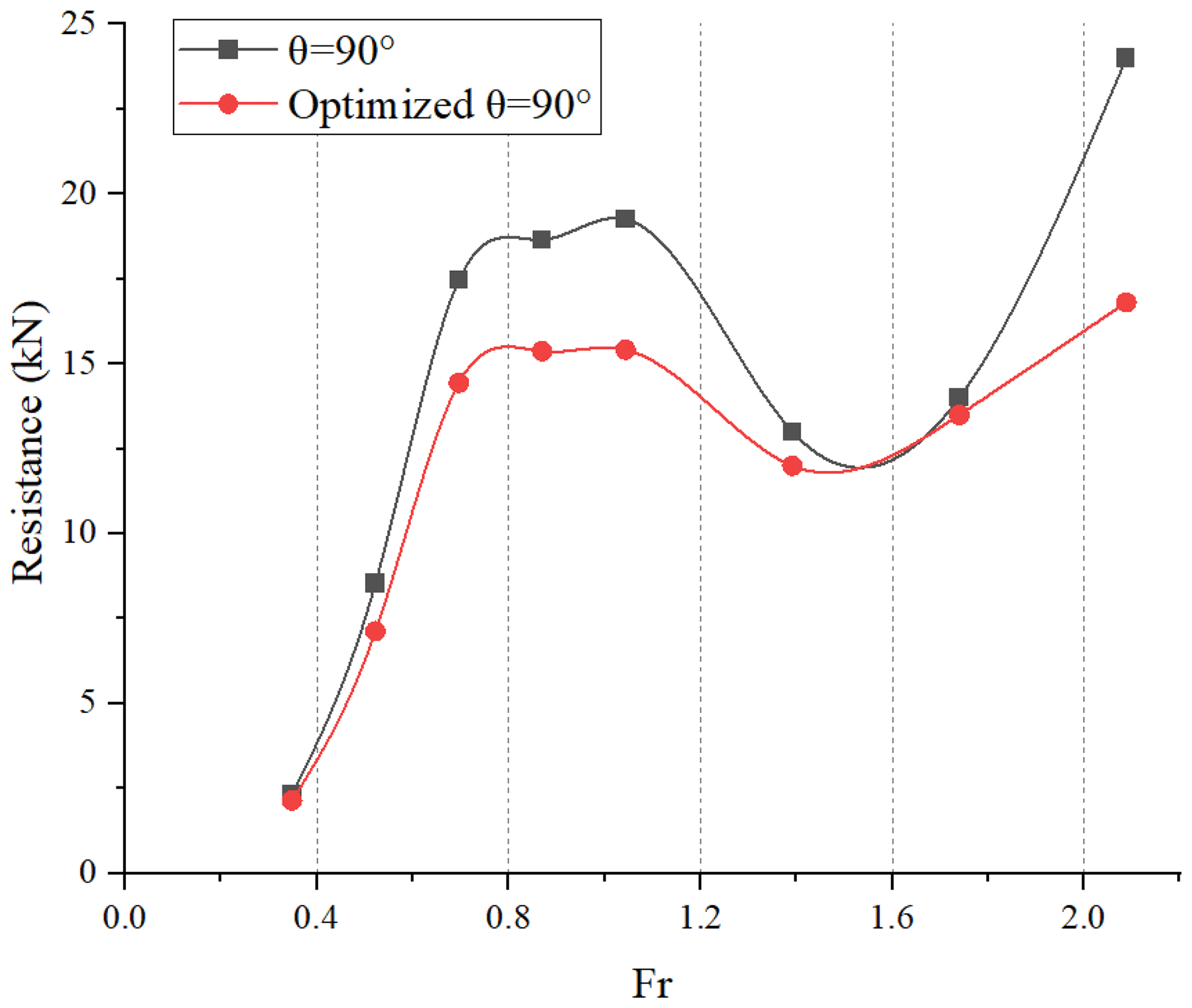
Figure 28 shows the resistance of the wheel well after optimization. When Fr<0.696, due to low speed, the resistance reduction effect is not obvious. When $\mathrm{0.696}<Fr<\mathrm{1.392}$, the vehicle enters into a planing regime, and it can be seen that the peak of resistance drops significantly. The maximum resistance reduction effect occurs at Fr = 1.044, which is expected to achieve 20 %. This indicates that optimization of the wheel well can significantly reduce the resistance of the HWAV during the transition stage, thus allowing the HWAV to reach a planing regime more quickly.

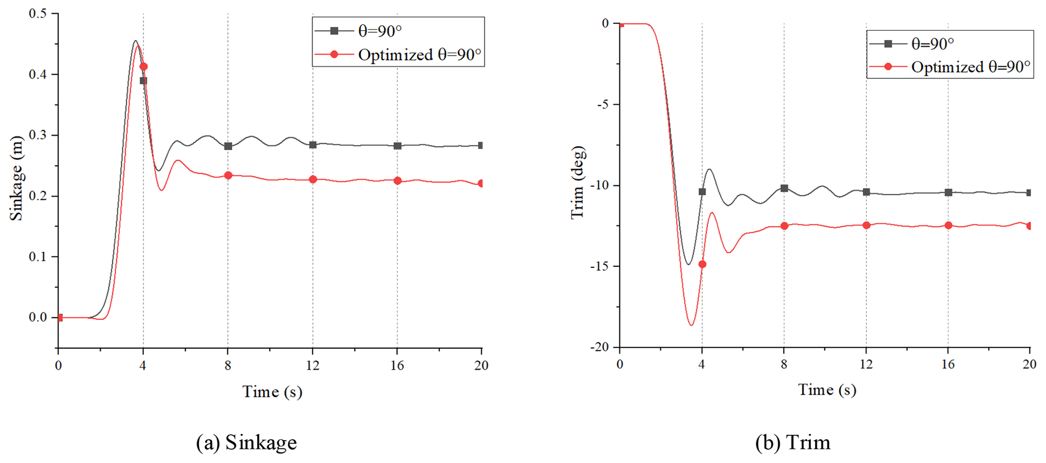
Figure 29 gives a clear picture of the comparison between the amplitude of sinkage and trim at Fr = 0.87. It can be seen that the sinkage is reduced and the trim is increased. When Fr = 0.87, the sinkage is reduced by about 21.9 % under an optimized wheel well compared with the wheel well without optimization, indicating that the optimized wheel well can decrease sinkage. By optimizing the wheel well, the water draft of the hull can be reduced, as can the resistance.

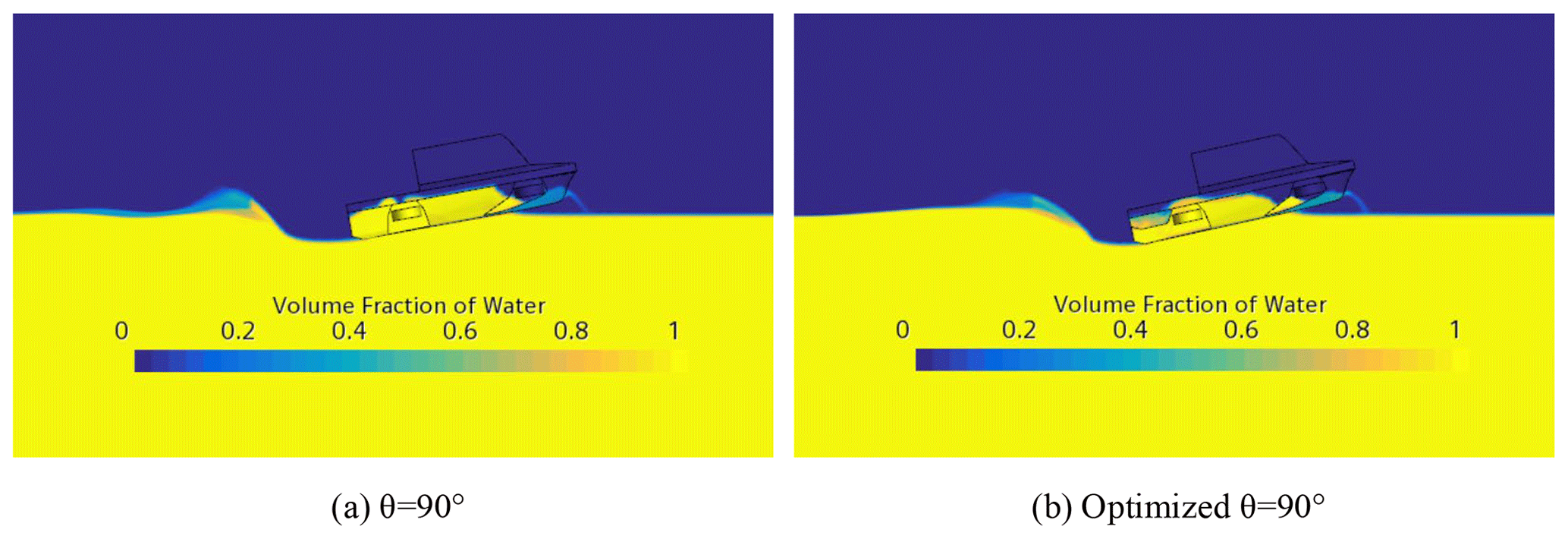
The gas–liquid phase diagram before and after the wheel-well optimization at Fr = 0.87 is shown in Fig. 30. The analysis of the water resistance characteristics of the HWAV shows that the wheel-well structure destroys the bottom line of the original hull, which complicates the contact between the hull and the water surface. In addition, after optimizing the wheel-well, pitch moment increases and leads to the bow rising and the stern falling.

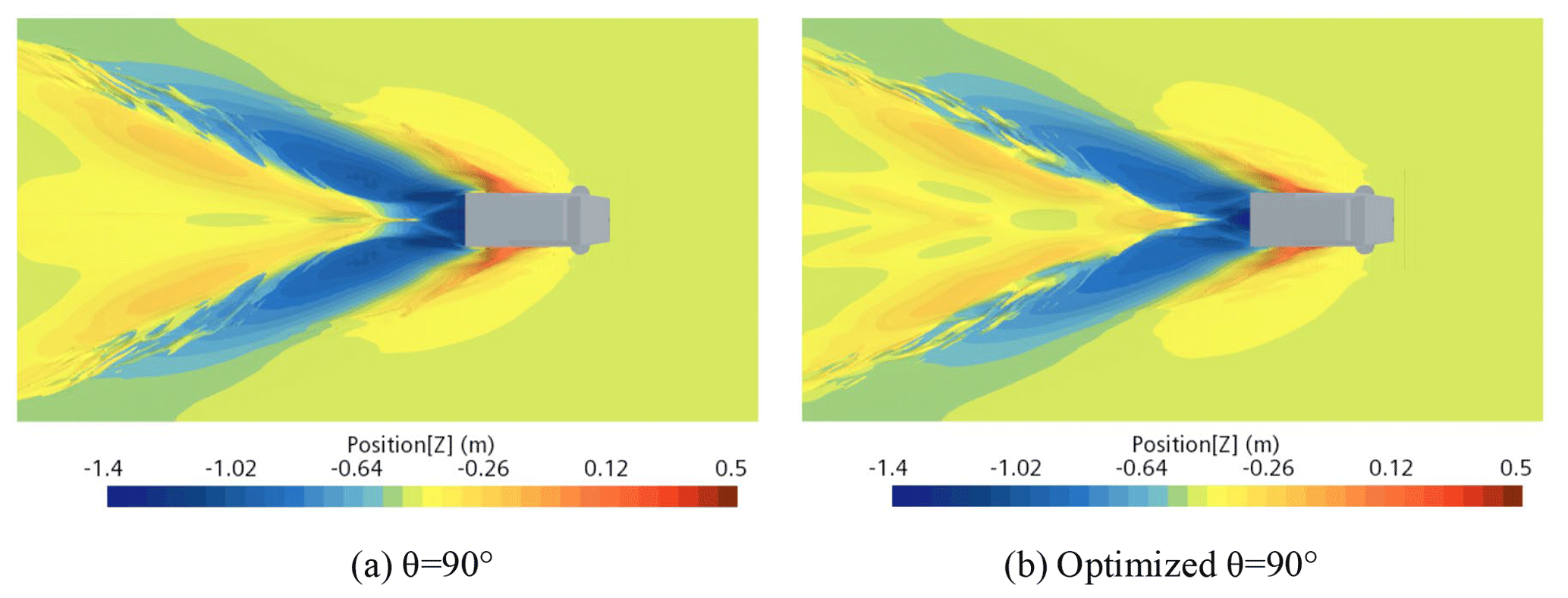
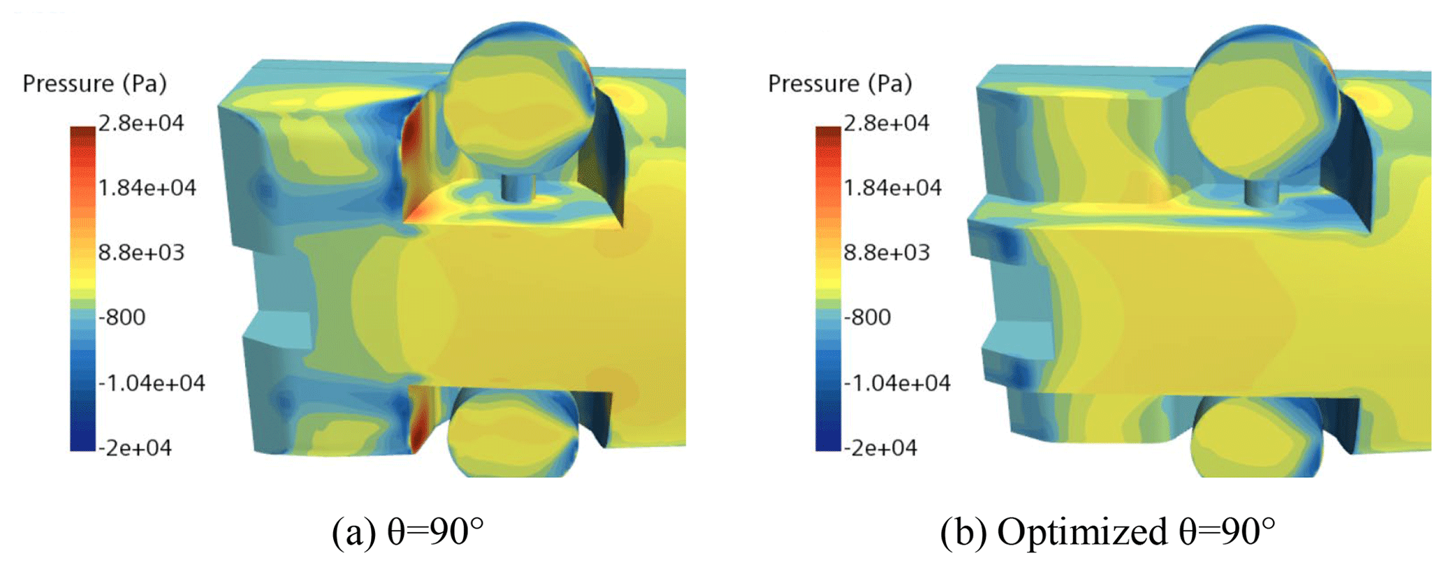
Figure 31 shows the wave pattern generated by an HWAV model sailing on water. The wave pattern is useful for analyzing ship resistance and wave-making interference between hulls. It can be observed that the wave-making region behind the stern became lankier, and the cocktail wake and cavity moved far away from the stern in optimized θ=90^∘ compared with θ=90^∘ at Fr=0.87.

As shown in Fig. 32, the pressure on the rear wheel well is significantly reduced before and after the wheel-well optimization at Fr=0.87, thus reducing the pressure of water flow on the bottom of the hull.

5 Conclusions

In this paper, hydrodynamic performance of the HWAV was analyzed using a numerical method, and the results show that the method can better simulate the hydrodynamic performance of the hull at different speeds, especially at high speeds. A numerical study was performed and the results were compared with experimental tests to ensure research reliability. Through the simulation and analysis, the following conclusions can be drawn:

1. The numerical method used in this study has high accuracy. The models including the turbulence model and VOF model, and the parameters (such as grid size and time step), are suitable for this large relative motion. In addition, overset mesh has considerable advantages in dealing with this problem.

2. The different wheels' flip angles have different effects on the HWAV. θ=30^∘ has the best resistance reduction at the peak of resistance with a maximum resistance reduction of 28 %. When the hull is under the planing regime, the maximum resistance reduction effect can be obtained by θ=90^∘. The hull can obtain the best heave and trim effect when Fr = 1.044 with θ=60^∘.

3. The influence of the wheel well on water resistance is relatively large, especially when the HWAV is under the transition stage of navigation. The maximum resistance reduction effect occurs in Fr = 1.044, which is expected to achieve 20 %. When Fr = 0.87, the sinkage was reduced by about 21.9 % under an optimized wheel well compared with the original wheel well. Therefore, the design of the wheel-well structure should be combined with the shape structure of the hull; the transition interface especially should be smooth as far as possible, to make the water flow smoothly and reduce resistance. The design of the vehicle shape structure should defer to the vehicle design ideas and to the theoretical technology of shipping and hydraulics.

Based on the work above, the influence of the wheel-well and wheel-retraction state on resistance and winding field can be further studied to provide some more guidance for the optimal design of the hull structure.