Synthesis of clearance for a kinematic pair to prevent an overconstrained linkage from becoming stuck

Mechanisms are prone to stuttering or even jamming due to the deformation of components, especially for overconstrained linkages for which geometric conditions must be strictly satisfied. In this paper, joint clearance is actively introduced to release the local constraint so that the linkages can still achieve general movement under the deformation of components. And a joint clearance model with a revolute joint (R-joint) is built. Based on the model, the minimum joint clearance introduced, which keeps mechanisms moving smoothly, is found when the components of the linkages have a certain deformation. The correctness of the proposed method is verified with a numerical case, and the optimal position for clearance introducing is analyzed. It opens up an important way to solve the phenomenon of stuttering or jamming in overconstrained linkages.

1 Introduction

Overconstrained linkages, which do not satisfy the Grübler–Kutzbach (G-K) criterion, are a kind of special mechanism and still have mobility due to the special geometric relationship between the joints and links. They have great application potential, especially in compact-deployable mechanisms, for their excellent rigidity and folding performance.

Over the past few decades, there have been many overconstrained linkages found. In Sarrus (1853), the first overconstrained linkage, the Sarrus linkage, was found. Since then, Bennett (1903), Bricard (1927), Myard (1931), and Goldberg (1943) linkages have been proposed – one after another. Based on those overconstrained linkages proposed, scholars have done a lot of research. Baker (1979) analyzed the intrinsic relationship between Bennett (1903), Goldberg (1943), and Myard (1931) and derived the complete closure equation for each linkage. In Song et al. (2014), Feng et al. (2017), and Yang and Chen (2021), the kinematic equation of the Bricard (1927) linkage was derived, and the bifurcation of motion under different geometric conditions was analyzed.

However, the strict geometric conditions of overconstrained linkages limit their practical application in spatial mechanisms (Mavroidis and Beddows, 1997; Chen, 2003), especially for the deployable structures constructed with overconstrained linkages that are expected to work in a space with a large change in temperature. To overcome this disadvantage, Yang et al. (2016) proposed a general truss transformation method to find their non-overconstrained forms and proved that the non-overconstrained equivalent linkages of the Bennett (1903) linkage and Myard (1931) 5R linkage are RSSR and RRSRR linkages, respectively. This approach can effectively alleviate the problem, but it is difficult to find the condition of non-overconstrained form (Yong et al., 2020).

In this paper, joint clearance is actively introduced to make overconstrained linkages movable, even when their components have deformations. For convenience, only one joint is allowed to introduce clearance, and the target is to find the minimum clearance that avoids too much wiggling. A brief description of the joint clearance model employed by the proposed method is first presented in Sect. 2, including an analysis of the relative motion between its journal and bearing. Section 3 presents the solving process of the minimum clearance in detail. In Sect. 4, a case study of the Bennett linkage is presented. And conclusions are given in Sect. 5 end the paper.

2 Kinematic modeling of the R-joint

2.1 Contact modes

A revolute joint (hereafter R-joint) is a kind of kinematic pair connecting two links and producing the relative rotation between the two links. An R-joint is composed of two components, a journal and a bearing, of which the axes coincide with the rotating axis if the clearance is small and negligible enough. Here, clearances are considered to evaluate their influence on the kinematics of spatial linkages, which will have the potential to prevent large deployable structures from getting stuck. The dimension parameters of a spatial R-joint with 3D clearances is shown in Fig. 1, and its radial and axial clearances can be obtained by Eq. (1).

$$\begin{array}{}\text{(1)}& C_{\mathrm{r}}={\displaystyle \frac{\mathrm{1}}{\mathrm{2}}}(D_Q-d_P),C_{\mathrm{a}}={\displaystyle \frac{\mathrm{1}}{\mathrm{2}}}(L_P-L_Q)\end{array}$$

For convenience, the journal and bearing are assumed to be rigid and without deformation during the process of motion, and the outer diameters of the joint and the bearing are assumed to be identical here. To reflect the relative motion of the two components, the joint is viewed as a base and the bearing as a moving part.

Figure 1 Spatial R-joint with radial and axial clearances.

There are, in total, three types of contact states between the journal and the bearing, namely surface contact, line contact, and point contact.

• a.

  When there is only transition for the bearing along its axis, then the end plane of the bearing will get into touch with the end face of the journal and its the surface contact state (see Fig. 2d).

• b.

  When there is only motion along the radial direction to the left, then it is named the line contact state. The bearing wall is fitted to the cylindrical surface of the journal (as shown in Fig. 2c).

• c.

  The third contact state will appear when there is a tilt angle between the axial and the radial axes. The cylindrical surface of the journal may be in contact with the bearing wall (as shown in Fig. 2a), and the upper (or lower) end face of the journal may get in contact with the end plane of the bearing (as shown in Fig. 2b), which is called the point contact.

Figure 2 Contact states, including (a) point contact I, (b) point contact II, (c) line contact, and (d) surface contact.

In addition, a combination of line contact and surface contact may occur.

In terms of large deployable mechanisms, they usually move at a low speed, which means that the journal and bearing are stably contacted during the whole motion. That is to say, there are at least two points that are in contact to guarantee stability. Significantly, coming into contact on the upper side or the lower side is the same due to the symmetry. Similarly, the bearing's tilting to the left or the right can be also viewed as being the same case.

Therefore, the contacting modes can be represented by one point indicating the position and posture of the axis of the bearing. For instance, the upper-right point of every subgraph in Fig. 2 is selected to indicate the contact between the journal and the bearing.

In such a manner, the contact modes can be divided into two cases, C₁ and C₃, when there is only the upward translation of the bearing (see Fig. 3a and b). C₁ represents the bearing wall that is in contact with the cylindrical surface of the journal, and C₃ represents the end plane of the bearing that is in contact with the end face of the journal. Figure 3c and d show two other cases, C₂ and C₄, that are similar to C₁ and C₃, respectively.

Figure 3 Contact modes, including (a) mode C₁, (b) mode C₃, (c) mode C₂, and (d) mode C₄.

In Fig. 4, P and Q are the center points of the journal and bearing, respectively, and s_Q​​​​​​​ represents the axial direction of the bearing. The fixed-coordinate system o-xyz is set up at point P, where the z axis is along the axial direction of the journal, and the x axis is located in the reference plane P₁, which is passing through the center of the journal, and the y axis is determined by the right-hand rule. It should be noticed that P₁ can be determined by the connecting link of the journal. As long as the movement of the bearing relative to the journal is known, the contact pose at every moment can be obtained.

Figure 4 Coordinate systems.

2.2 Kinematic description of the relative motion and transformation matrix

There is a tendency to move in five other directions when there are radial and axial clearances in an R-joint. In order to describe the movements between the journal and the bearing clearly, the movements are analyzed in steps as follows.

Figure 5 Relative movement states, including the (a) initial state, (b) transition state, and (c) inclination state.

Initially, the point Q and vector s_Q values are assumed to coincide with P and the z axis, respectively, as shown in Fig. 5a. First, the bearing translates t_x, t_y, and t_z along the direction of three axes, and the direction of translation is $\mathit{\lambda }=\arctan t_y/t_x$. For convenience, the plane crossing the axes of the journal and the bearing is named the transition plane P₂, as shown in Fig. 5b. And P₂ and P₁ will coincide when the two axes are collinear. So, the homogeneous transformation matrix can be obtained as follows:

$$\begin{array}{}\text{(2)}& {\mathbf{T}}_{xyz}=\left[\begin{array}{cccc}\mathrm{1}& \mathrm{0}& \mathrm{0}& t_x\\ \mathrm{0}& \mathrm{1}& \mathrm{0}& t_y\\ \mathrm{0}& \mathrm{0}& \mathrm{1}& t_z\\ \mathrm{0}& \mathrm{0}& \mathrm{0}& \mathrm{1}\end{array}\right],\end{array}$$

where $\sqrt{t_x^{\mathrm{2}}+t_y^{\mathrm{2}}}\in [\mathrm{0},C_{\mathrm{r}}],t_z\in [-C_{\mathrm{a}},C_{\mathrm{a}}]$.

The bearing has 2π possible azimuths inclined to s_Q because of its axial symmetry. So, to determine the final posture of the bearing, the rotating angle ξ (see Fig. 6a) and the inclination angle γ (see Fig. 6b) are defined to determine the inclination azimuth and the inclination angle, respectively. P₂ is rotated ξ around s_Q and then intersects with the bearing at line $l_{N_{\mathrm{i}}}$, which is point N_i (as shown in Fig. 6a), where point N_i is on the plane xoy, and its rotation matrix is as follows:

$$\begin{array}{}\text{(3)}& \mathbf{Rot}({\mathit{s}}_Q,\mathit{\xi })=\left[\begin{array}{cccc}\cos \left(\mathit{\xi }\right)& -\sin \left(\mathit{\xi }\right)& \mathrm{0}& \mathrm{0}\\ \sin \left(\mathit{\xi }\right)& \cos \left(\mathit{\xi }\right)& \mathrm{0}& \mathrm{0}\\ \mathrm{0}& \mathrm{0}& \mathrm{1}& \mathrm{0}\\ \mathrm{0}& \mathrm{0}& \mathrm{0}& \mathrm{1}\end{array}\right].\end{array}$$

And the plane is called the inclination plane P₃, which is formed by the z axis and the line $l_{N_{\mathrm{i}}}$, as shown in Fig. 5c. Finally, the bearing is rotated around the line Ps, which is the normal line of P₃ (as shown in Fig. 6 by the angle γ) which then contacts the journal. The process of solving the direction vector of Ps is as follows.

Figure 6 Incline plane schematic, with the (a) top view and (b) front view.

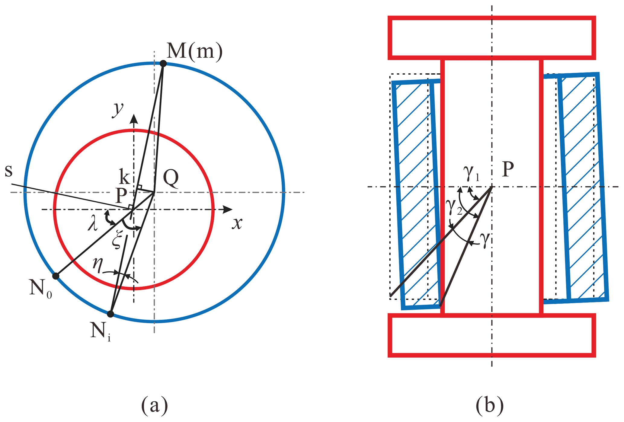
From the description above, the point can be obtained as follows:

$$\begin{array}{ll}{\displaystyle }{\mathit{N}}_{\mathrm{i}}=& {\displaystyle }\left({\mathbf{T}}_{xyz}\mathbf{Rot}\right({\mathit{s}}_Q,\mathit{\xi }){)}^{-\mathrm{1}}\\ {\displaystyle }& {\displaystyle }\times {\left[\begin{array}{cccc}{R}_Q\cos (\mathit{\pi }+\mathit{\lambda })& R_Q\sin (\mathit{\pi }+\mathit{\lambda })& -t_z& \mathrm{1}\end{array}\right]}^{\mathrm{T}}\\ \text{(4)}& {\displaystyle }=& {\displaystyle }{\left[\begin{array}{cccc}{t}_z-R_Q\cos (\mathit{\lambda }+\mathit{\xi })& t_y-R_Q\sin (\mathit{\lambda }+\mathit{\xi })& \mathrm{0}& \mathrm{1}\end{array}\right]}^{\mathrm{T}}.\end{array}$$

The line Ps is perpendicular to both the z axis and the line PN_i, while

$$\begin{array}{}\text{(5)}& \begin{array}{rl}P{\mathit{N}}_{\mathrm{i}}=& N_{\mathbf{i}}-P\\ =& {\left[\begin{array}{cccc}{t}_x-R_Q\cos (\mathit{\lambda }+\mathit{\xi })& t_y-R_Q\sin (\mathit{\lambda }+\mathit{\xi })& \mathrm{0}& \mathrm{0}\end{array}\right]}^{\mathrm{T}}\end{array},\end{array}$$

so that

$$\begin{array}{}\text{(6)}& \begin{array}{rl}\mathit{P}\mathit{s}=& P{N}_{\mathrm{i}}\times {\left[\begin{array}{cccc}\mathrm{0}& \mathrm{0}& \mathrm{1}& \mathrm{0}\end{array}\right]}^{\mathrm{T}}\\ =& {\left[\begin{array}{cccc}{t}_y-R_Q\sin (\mathit{\lambda }+\mathit{\xi })& R_Q\cos (\mathit{\lambda }+\mathit{\xi })-t_z& \mathrm{0}& \mathrm{0}\end{array}\right]}^{\mathrm{T}}\end{array},\end{array}$$

and its unit vector is

$$\begin{array}{}\text{(7)}& {\mathit{e}}_{Ps}={\displaystyle \frac{{\left[\begin{array}{cccc}{t}_y-R_Q\sin (\mathit{\lambda }+\mathit{\xi })& R_Q\cos (\mathit{\lambda }+\mathit{\xi })-t_x& \mathrm{0}& \mathrm{0}\end{array}\right]}^{\mathrm{T}}}{\sqrt{t^{\mathrm{2}}-\mathrm{2}t{R}_Q\cos \mathit{\xi }+R_Q^{\mathrm{2}}}}},\end{array}$$

where $t=\sqrt{t_x^{\mathrm{2}}+t_y^{\mathrm{2}}}$.

The transformation matrix for the rotating the angle γ around the line Ps is as follows (Cai, 2009):

$$\begin{array}{c}{\displaystyle }\mathbf{Rot}({\mathit{e}}_{Ps},\mathit{\gamma })=\\ \text{(8)}& {\displaystyle }\left[\begin{array}{cccc}{e}_x{e}_x\text{vers}\mathit{\gamma }+\mathrm{c}\mathit{\gamma }& e_y{e}_x\text{vers}\mathit{\gamma }-e_z\mathrm{s}\mathit{\gamma }& e_z{e}_x\text{vers}\mathit{\gamma }+e_y\mathrm{s}\mathit{\gamma }& \mathrm{0}\\ e_x{e}_y\text{vers}\mathit{\gamma }+e_z\mathrm{s}\mathit{\gamma }& e_y{e}_y\text{vers}\mathit{\gamma }+\mathrm{c}\mathit{\gamma }& e_z{e}_y\text{vers}\mathit{\gamma }+e_x\mathrm{s}\mathit{\gamma }& \mathrm{0}\\ e_x{e}_z\text{vers}\mathit{\gamma }-e_y\mathrm{s}\mathit{\gamma }& e_y{e}_z\text{vers}\mathit{\gamma }+e_x\mathrm{s}\mathit{\gamma }& e_z{e}_z\text{vers}\mathit{\gamma }+\mathrm{c}\mathit{\gamma }& \mathrm{0}\\ \mathrm{0}& \mathrm{0}& \mathrm{0}& \mathrm{1}\end{array}\right],\end{array}$$

where $\text{vers}\mathit{\gamma }=\mathrm{1}-\mathrm{c}\mathit{\gamma },\mathrm{c}\mathit{\gamma }=\cos \mathit{\gamma },\mathrm{s}\mathit{\gamma }=\sin \mathit{\gamma }$, and γ can be solved as follows.

In $\mathrm{\Delta }P\stackrel{\mathrm{‾}}{Q}{N}_{\mathrm{i}}$ (as shown in Fig. 6), the following can be known from the cosine law:

$$\begin{array}{}\text{(9)}& L_{\mathrm{i}}={\stackrel{\mathrm{‾}}{PN}}_{\mathrm{i}}=\sqrt{r_Q^{\mathrm{2}}+t^{\mathrm{2}}-\mathrm{2}{r}_{Q}t\cos \mathit{\xi }},\end{array}$$

where $\stackrel{\mathrm{‾}}{Q}$ represents the projection of Q in the fixed-coordinate system, and r_Q takes $d_Q/\mathrm{2}$ when the inner diameter of the bearing is in contact and $D_Q/\mathrm{2}$ when the outer diameter is in contact.

From Fig. 6b, the following can be obtained:

$$\begin{array}{}\text{(10)}& \mathit{\gamma }={\mathit{\gamma }}_{\mathrm{2}}-{\mathit{\gamma }}_{\mathrm{1}}.\end{array}$$

When the contact mode is C₁,

$$\begin{array}{}\text{(11)}& \begin{array}{rl}& {\mathit{\gamma }}_{{\mathrm{1}}_{C\mathrm{1}}}=\arctan {\displaystyle \frac{\frac{L_Q}{\mathrm{2}}+t_z}{L_{\mathrm{i}}}}\\ & {\mathit{\gamma }}_{{\mathrm{2}}_{C\mathrm{1}}}=\arccos {\displaystyle \frac{r_P}{\sqrt{L_{\mathrm{i}}^{\mathrm{2}}+{\left(\frac{L_Q}{\mathrm{2}}+t_z\right)}^{\mathrm{2}}}}},\end{array}\end{array}$$

where r_P represents the radius of the journal, and $r_P=d_P/\mathrm{2}$.

When the contact mode is C₂, then

$$\begin{array}{}\text{(12)}& \begin{array}{rl}& {\mathit{\gamma }}_{{\mathrm{1}}_{C\mathrm{2}}}={\mathit{\gamma }}_{{\mathrm{1}}_{C\mathrm{1}}}\\ & {\mathit{\gamma }}_{{\mathrm{2}}_{C\mathrm{2}}}=\arcsin {\displaystyle \frac{L_P}{\mathrm{2}\sqrt{L_{\mathrm{i}}^{\mathrm{2}}+{\left(\frac{L_Q}{\mathrm{2}}+t_z\right)}^{\mathrm{2}}}}}.\end{array}\end{array}$$

When the contact mode is C₃ in $\mathrm{\Delta }P\stackrel{\mathrm{‾}}{Q}{N}_{\mathrm{i}}$ (shown in Fig. 6a), then the following can be known from the sine law:

$$\begin{array}{}\text{(13)}& \mathit{\eta }=\arcsin {\displaystyle \frac{t\sin \mathit{\xi }}{L_{\mathrm{i}}}}.\end{array}$$

In $\mathrm{\Delta }\stackrel{\mathrm{‾}}{Q}{N}_{\mathrm{i}}M$, the following can be known from the cosine law:

$$\begin{array}{}\text{(14)}& \stackrel{\mathrm{‾}}{M{N}_{\mathrm{i}}}=\mathrm{2}{r}_{Q}t\cos \mathit{\eta }.\end{array}$$

Thus,

$$\begin{array}{}\text{(15)}& \stackrel{\mathrm{‾}}{PM}=\stackrel{\mathrm{‾}}{M{N}_{\mathrm{i}}}-\stackrel{\mathrm{‾}}{P{N}_{\mathrm{i}}}=\mathrm{2}{r}_Q\cos \mathit{\eta }-L_{\mathrm{i}}.\end{array}$$

Substituting Eq. (9) into Eq. (15) gives the following:

$$\begin{array}{}\text{(16)}& \begin{array}{rl}& {\mathit{\gamma }}_{{\mathrm{1}}_{C\mathrm{3}}}=\arctan {\displaystyle \frac{\frac{L_Q}{\mathrm{2}}-t_z}{PM}}\\ & {\mathit{\gamma }}_{{\mathrm{2}}_{C\mathrm{3}}}=\arccos {\displaystyle \frac{r_P}{\sqrt{P{M}^{\mathrm{2}}+{\left(\frac{L_Q}{\mathrm{2}}-t_z\right)}^{\mathrm{2}}}}}.\end{array}\end{array}$$

When the contact mode is C₄, then

$$\begin{array}{}\text{(17)}& \begin{array}{rl}& {\mathit{\gamma }}_{{\mathrm{1}}_{C\mathrm{4}}}={\mathit{\gamma }}_{{\mathrm{1}}_{C\mathrm{3}}}\\ & {\mathit{\gamma }}_{{\mathrm{2}}_{C\mathrm{4}}}=\arcsin {\displaystyle \frac{L_P}{\mathrm{2}\sqrt{P{M}^{\mathrm{2}}+{\left(\frac{L_Q}{\mathrm{2}}-t_z\right)}^{\mathrm{2}}}}}.\end{array}\end{array}$$

Thus, the transformation matrix of relative motion between the bearing and the journal is as follows:

$$\begin{array}{}\text{(18)}& {\mathbf{T}}_{P\left(Q\right)}={\mathbf{T}}_{xyz}\cdot \mathbf{Rot}(r_Q,\mathit{\xi })\cdot \mathbf{Rot}({\mathit{e}}_{Ps},\mathit{\gamma }).\end{array}$$

The actual contact mode can be determined when the minimum of γ is solved at every posture. And all possible contact poses between the journal and the bearing can be obtained if the dimension of the R-joint is known.

3 Synthesis of clearance dimensions

The continuous movable condition of a linkage is that each input has a corresponding output. The geometric conditions of overconstrained linkages are not satisfied any more when the components have a deformation, which would cause linkage to become stuck or even to become rigid. Proper joint clearance will remove the need for the geometric conditions and make it possible for the linkages to move.

The larger the value of the clearance introduced, the higher tolerance of the range of deformation for the components can be – in theory. However, as clearance would cause fluctuations and reduce motion accuracy, it cannot be enlarged too much. So, the target is to find the minimum value of a joint clearance below which the mechanism could not work for the whole working period; i.e., the linkages' critical condition is that there is only one set of inputs and outputs satisfying a one-to-one correspondence at some particular position.

Figure 7 Linkages are separated into the (a) input part and (b) output part.

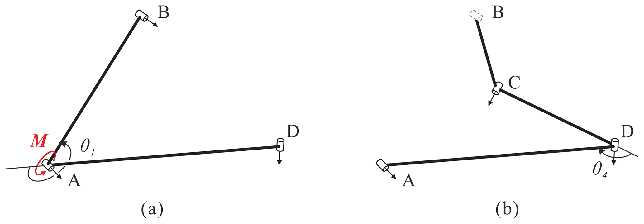
Due to the property of a single degree of freedom, single-loop, overconstrained linkages are divided into two parts, namely input and output ones, based on the location introduced for joint clearance, as shown in Fig. 7. The minimum clearance-introducing value can be obtained by judging whether the linkages meet continuous movable and critical conditions. Besides, the location of the clearance introducing does not include the input and output joints. And the bisection method is used to adjust the clearance in order to approach it constantly. The flowchart is shown in Fig. 8, and the specific steps are as follows.

• Step 1. The parameters of overconstrained linkages are brought into the linkages' kinematic equation to determine the range of the kinematic angle. The linkages are divided into input and output parts, based on position of joints clearance, and the journal is fixed at the input part and the bearing to the output. The position and posture about the end of two parts are analyzed by the Denavit–Hartenberg (D-H) method, as follows:

  $$\begin{array}{}\text{(19)}& {\displaystyle }\mathit{P}={\mathbf{T}}_{\text{in}}{\left[\begin{array}{cccc}\mathrm{0}& \mathrm{0}& \mathrm{0}& \mathrm{1}\end{array}\right]}^{\mathrm{T}},\text{(20)}& {\displaystyle }{\mathit{S}}_P={\mathbf{T}}_{\text{in}}{\left[\begin{array}{cccc}\mathrm{0}& \mathrm{0}& \mathrm{1}& \mathrm{0}\end{array}\right]}^{\mathrm{T}},\text{(21)}& {\displaystyle }\mathit{Q}={\mathbf{T}}_{\text{out}}{\left[\begin{array}{cccc}\mathrm{0}& \mathrm{0}& \mathrm{0}& \mathrm{1}\end{array}\right]}^{\mathrm{T}},\text{(22)}& {\displaystyle }{\mathit{S}}_Q={\mathbf{T}}_{\text{out}}{\left[\begin{array}{cccc}\mathrm{0}& \mathrm{0}& \mathrm{1}& \mathrm{0}\end{array}\right]}^{\mathrm{T}}.\end{array}$$

  The angle γ_c, the horizontal and vertical distance between the end of the input and output, can be deduced by Eqs. (23), (24), and (25), respectively.

  $$\begin{array}{}\text{(23)}& {\displaystyle }{\mathit{\gamma }}_c=\arccos \left({\displaystyle \frac{S_P\times S_Q}{\left|S_P\right|\times \left|S_Q\right|}}\right)\text{(24)}& {\displaystyle }{t}_c=\left|S_P\right|\cos \mathit{\zeta }\text{(25)}& {\displaystyle }{t}_{zc}=\left|S_P\right|\sin \mathit{\zeta },\end{array}$$

  where ζ represents the angle between S_P and the vector r_PQ.

• Step 2. The motion variables γ, t, and t_z, as well as the radial and axial clearances C_a and C_r, can be obtained from the kinematic pair model when the dimension parameters of the kinematic pair are known. And the lower and upper limits of bisection method are 0 and C_r, respectively. So, the middle is as follows:

  $$\begin{array}{}\text{(26)}& m={\displaystyle \frac{a+b}{\mathrm{2}}},\end{array}$$

  where a and b represent the lower and upper limits, respectively.

• Step 3. Find out all output angles that meet the constraints and correspond to input. It is because of the existence of clearance that one input corresponds to multiple outputs. It thus needs the expansion of the range of output angles to find them all. And the constraints condition is as follows:

  $$\begin{array}{}\text{(27)}& \begin{array}{rl}& {\mathit{\gamma }}_c=\mathit{\gamma }\\ & t_c=t\\ & t_{zc}=t_z.\end{array}\end{array}$$

• Step 4. If the linkages satisfy the continuous movable condition, then b=m, and the middle meets in Eq. (8). If not, then a=m.

• Step 5. The value is considered to have been found when the result meets conditions 1 and 2. If not, then repeat Steps 2 to 4 until the result is found. Condition 1 is the critical condition mentioned above. Condition 2 is $|a-b|\le d$, where d is the precision of the judgment and should be less than the step distance of kinematic pair model; i.e., the difference between the upper and lower limits is already less than the step distance of kinematic pair model, and the result can be used as the final value.

Figure 8 The flowchart of minimum clearance.

The precision and efficiency of the numerical iterative method are affected by the step distance of the variable. So, two steps are adopted to find the final results, namely preliminary search and final search, where the preliminary search has a larger step distance, and the final search has a smaller one.

4 Applications and numerical analysis: Bennett linkage

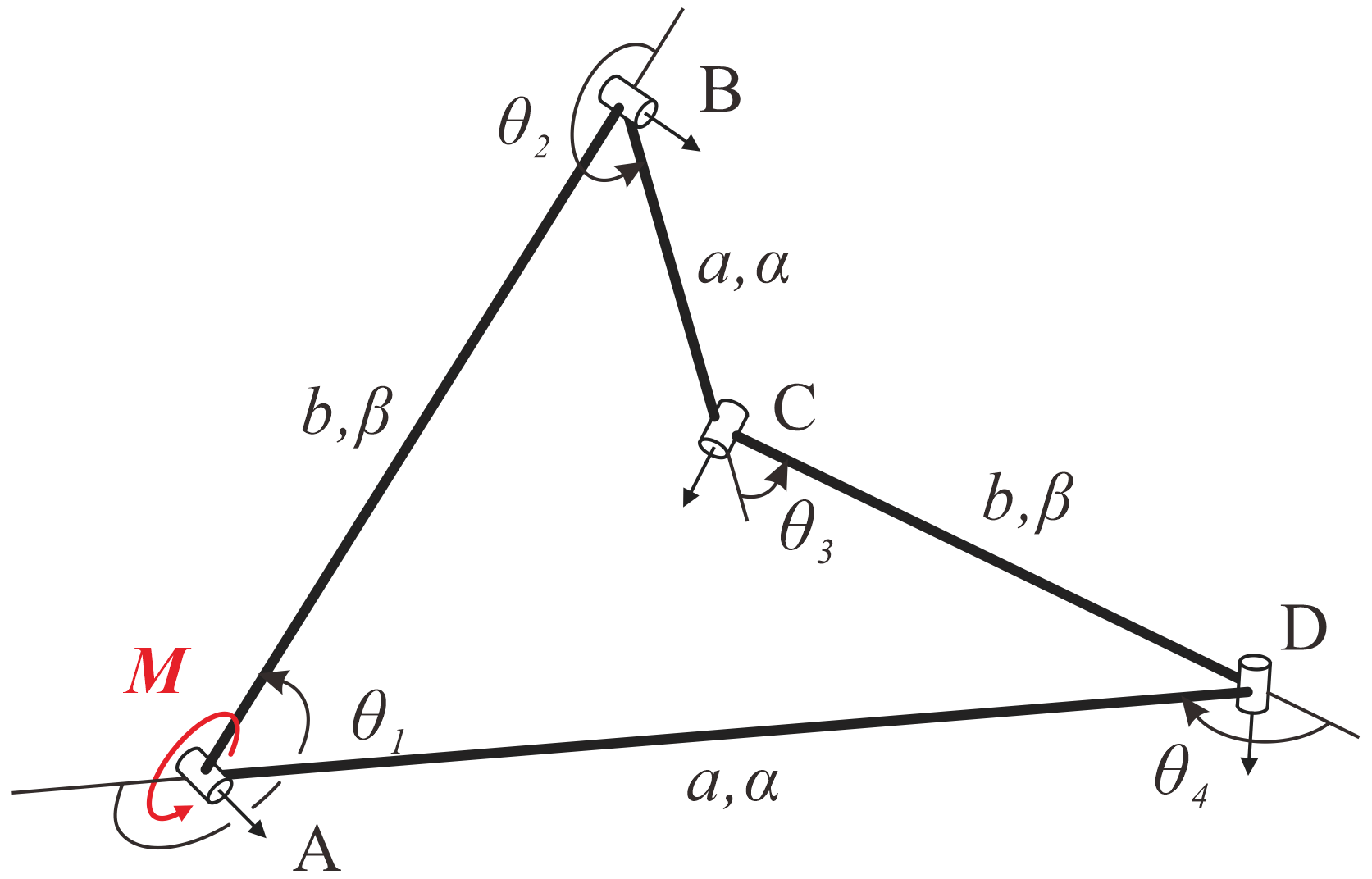
In this section, the Bennett linkage is used as an example to analyze the minimum clearance introduced when it has the deformation of certain components. The Bennett linkage is a typical spatially overconstrained mechanism with the least number of links (Yang et al., 2020; as shown in Fig. 9), and its geometric condition without joint clearances is as follows (Bennett, 1903):

$$\begin{array}{}\text{(28)}& {\displaystyle \frac{\sin \mathit{\alpha }}{a}}={\displaystyle \frac{\sin \mathit{\beta }}{b}},\end{array}$$

and the relationships among all the variables are

$$\begin{array}{}\text{(29)}& \begin{array}{rl}& {\mathit{\theta }}_{\mathrm{1}}+{\mathit{\theta }}_{\mathrm{3}}=\mathrm{2}\mathit{\pi },{\mathit{\theta }}_{\mathrm{2}}+{\mathit{\theta }}_{\mathrm{4}}=\mathrm{2}\mathit{\pi }\\ & \tan {\displaystyle \frac{{\mathit{\theta }}_{\mathrm{1}}}{\mathrm{2}}}\tan {\displaystyle \frac{{\mathit{\theta }}_{\mathrm{2}}}{\mathrm{2}}}={\displaystyle \frac{\sin \frac{\mathrm{1}}{\mathrm{2}}(\mathit{\beta }+\mathit{\alpha })}{\sin \frac{\mathrm{1}}{\mathrm{2}}(\mathit{\beta }-\mathit{\alpha })}}.\end{array}\end{array}$$

Figure 9 Bennett linkage.

4.1 Numerical results

This paper takes the commonly used space material, titanium alloy (TC4), as an example for analysis. And the geometric parameters and the components' deformation of the Bennett linkage are listed in Table 1, where the components' deformation is obtained by a liner thermal expansion formula and Hooke's law (Hongwen, 2017). Here, the limit of the temperature difference in the space ΔT=200 ^∘C is taken as an example for analysis.

Table 1 Related parameters of the Bennett linkage.

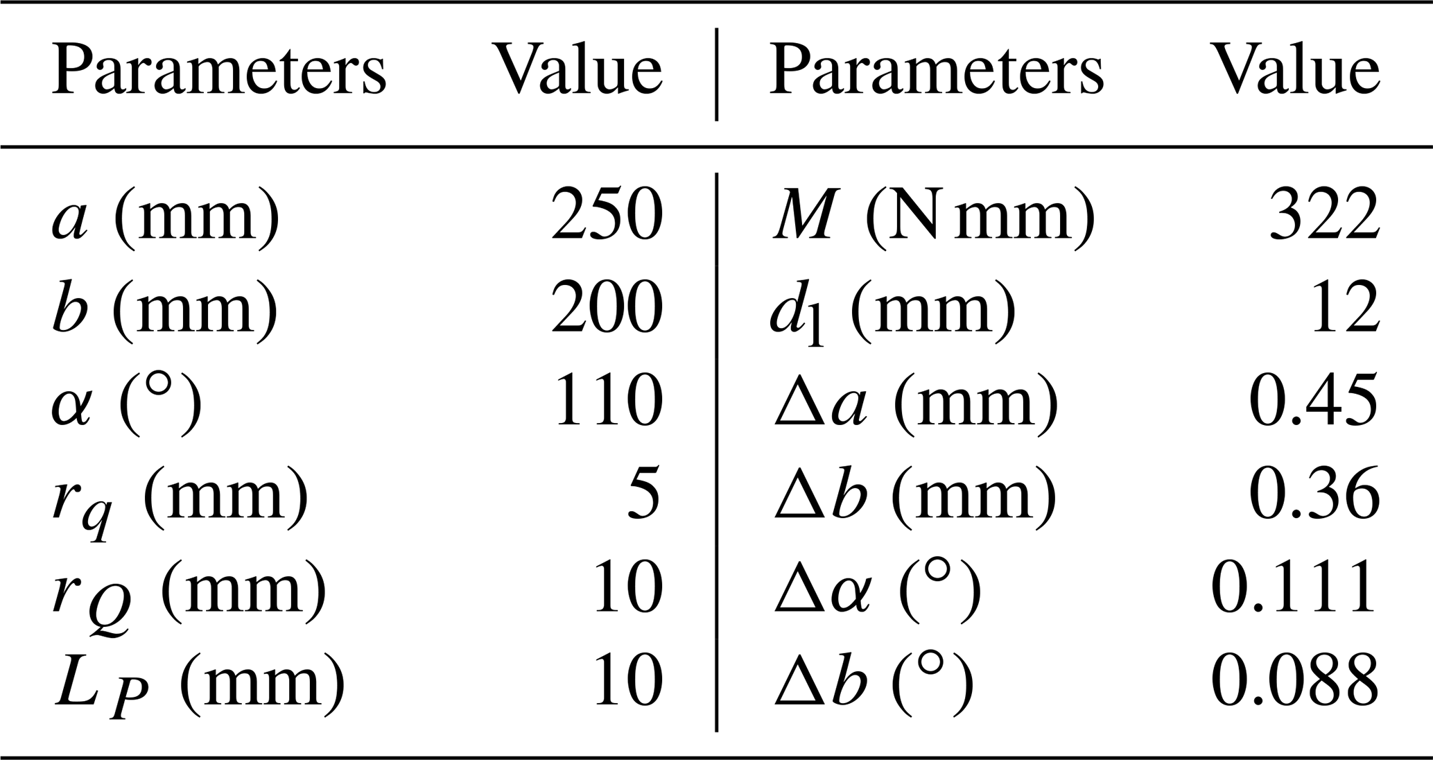
M, d_l, and Δi represent the torque, the link diameter, and the deformation of i, respectively.

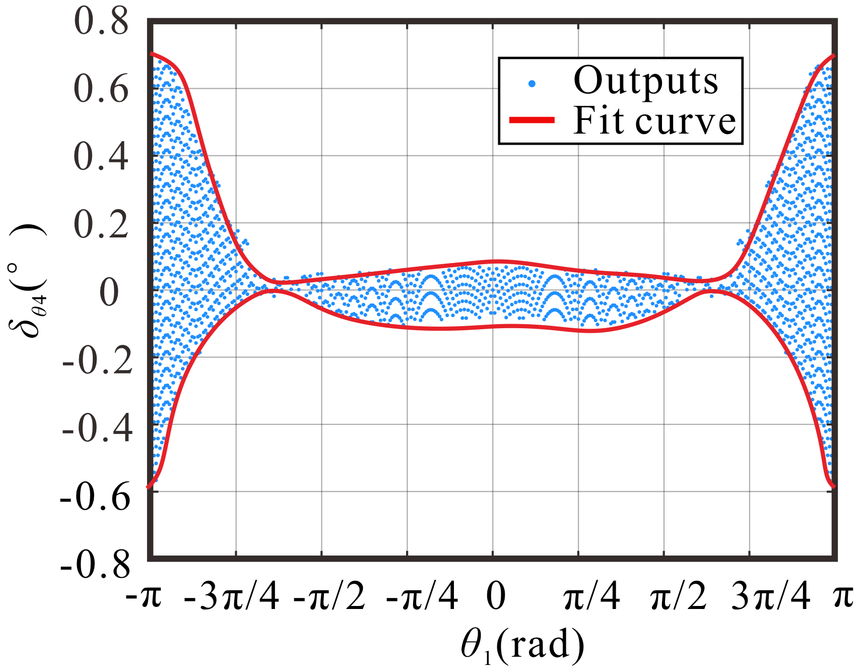
According to the analysis, it requires at least 0.379 mm clearance at joint B to keep the Bennett linkage's motion smooth, and it is the same at joint C. So, introducing clearance at joint B or joint C is equivalent in the Bennett linkage. Figure 10 shows the fluctuation in the output angle after the introduction of clearance in joint B and the components' deformation. It shows a trend of high clearance on both sides, it is low in the middle in each half-motion cycle, and the fluctuation is close to 0 when the input is around $\pm \mathrm{109}{}^{\circ }$. In addition, the biggest fluctuation in the output is less than 0.8^∘, and it only occurs when the input link is approximately parallel (or collinear) to the frame, which can also be reduced further by choosing material with greater rigidity.

Figure 10 The fluctuation in the output angle.

4.2 Verification of the method

The fluctuation tends to 0, which indicates that the position around 109^∘ meets the critical condition of the Bennett linkage. Therefore, it is necessary to verify that the current input corresponds to only one output. Taking ${\mathit{\theta }}_{\mathrm{1}}=\mathrm{109}{}^{\circ }$ into the kinematics can obtain the output ${\mathit{\theta }}_{\mathrm{40}}=-\mathrm{107.975}{}^{\circ }$. To verify the output's uniqueness, it is necessary to add a step to the output, and the step of the output is 0.025^∘, i.e., ${\mathit{\theta }}_{\mathrm{41}}=-\mathrm{107.95}{}^{\circ }$. In the end of the input part, it has a workspace due to the joint clearance, and the end of the output part also has a workspace when the kinematic angle θ₃ has no limit. And Fig. 11 shows the relationship of the two workspaces.

Figure 11 Relationship of the workspace between input and output parts when ${\mathit{\theta }}_{\mathrm{1}}=\mathrm{109}{}^{\circ }$. (a) ${\mathit{\theta }}_{\mathrm{40}}=-\mathrm{107.975}{}^{\circ }$. (b) ${\mathit{\theta }}_{\mathrm{41}}=-\mathrm{107.95}{}^{\circ }$.

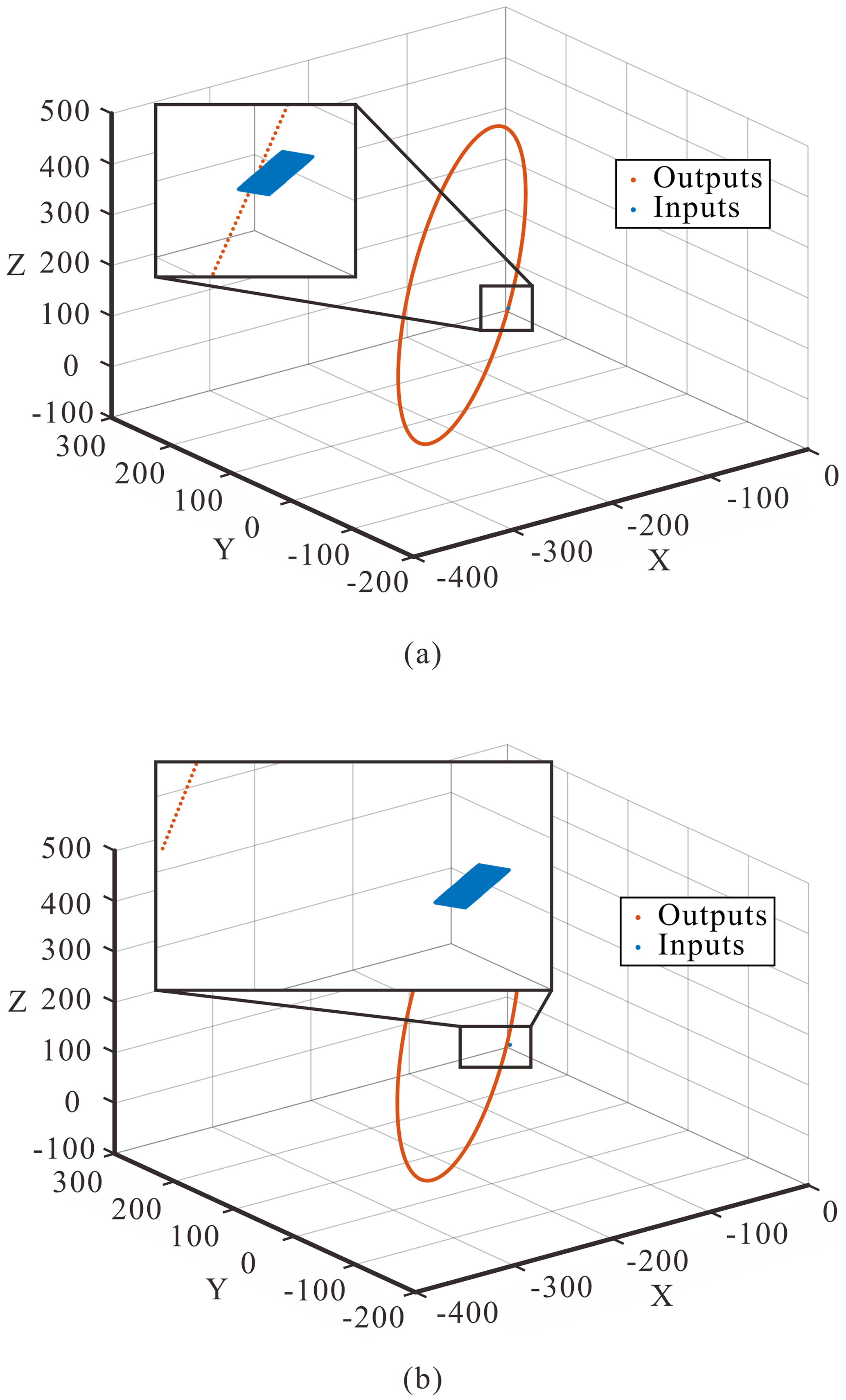
This means that the current input and output have a corresponding relationship when the two workspaces intersect. And it can be seen from Fig. 11a that the two workspaces are fairly close, and the minimum distance is 0.0191 mm, which can be regarded as an intersection. However, the minimum distance between the two workspaces is 20.2552 mm (Fig. 11b), which cannot be ignored. So, the current input corresponds to a small range of output; i.e., the introduced clearance allows the Bennett linkage to meet the critical condition at the present position. Therefore, the result is the minimum clearance introduced under the current deformation of the components.

5 Conclusions

In this paper, we present a joint clearance model with an R-joint to analyze the kinematic characteristics of overconstrained linkages with joint clearance and the deformation of components. According to the influence of the joint clearance for linkages, we propose a method that actively introduces joint clearance to alleviate the linkage-jamming phenomenon caused by the component deformation of overconstrained linkages and verify its correctness with a numerical example. This method is a general one for single-loop linkages, and the linkages can be cut hypothetically, as in the processing of the example, and then the input part and the output one could be analyzed similarly. It provides a new idea and direction for solving the problem of stuttering or jamming.

Taking the Bennett linkage as an example, the optimal position to introduce clearance is analyzed, and the result shows that the clearance introduced at joint B is the same as joint C under the same deformation. That is, both joint B and joint C can meet the critical conditions of the Bennett linkage with a smaller joint clearance, so that the Bennett linkage can achieve the alleviation of a freezing problem under smaller fluctuations in the output. However, it may be different in other overconstrained linkages. In future work, it is necessary to study the relationship between the size of the clearance introduced and the deformation of the component, so as to apply the method more effectively.