the Creative Commons Attribution 4.0 License.
the Creative Commons Attribution 4.0 License.
 | 28 Nov 2022
Instability load analysis of a telescopic boom for an all-terrain crane
Jinshuai Xu
Yingpeng Zhuo
Gang Wang
Tianjiao Zhao
Tianyu Wang
The instability load for the telescopic boom of an all-terrain crane is investigated in this paper. Combined with structural characteristics of the telescopic boom, each boom section is divided into several substructures, and the fixed-body coordinate system of each substructure is established based on the co-rotational method. A 3D Euler–Bernoulli eccentric beam element of the telescopic boom is derived. On the premise of considering the discretization of gravity and wind load, internal degrees of freedom of the substructure are condensed to the boundary nodes, forming a geometrical nonlinear super element. According to the nesting mode of the telescopic boom, a constraint way is established. The unstressed original length of the guy rope is calculated with a given preload so as to establish the equilibrium equations of the boom system with the external force of the guy rope and the corresponding tangent stiffness matrix. Regarding the above work, a new method for calculating the structural equilibrium path and instability load of telescopic boom structure is presented by solving the governing equations in a differential form. Finally, the method is validated by examples with different features.
- Article
(7824 KB) - Full-text XML
- BibTeX
- EndNote


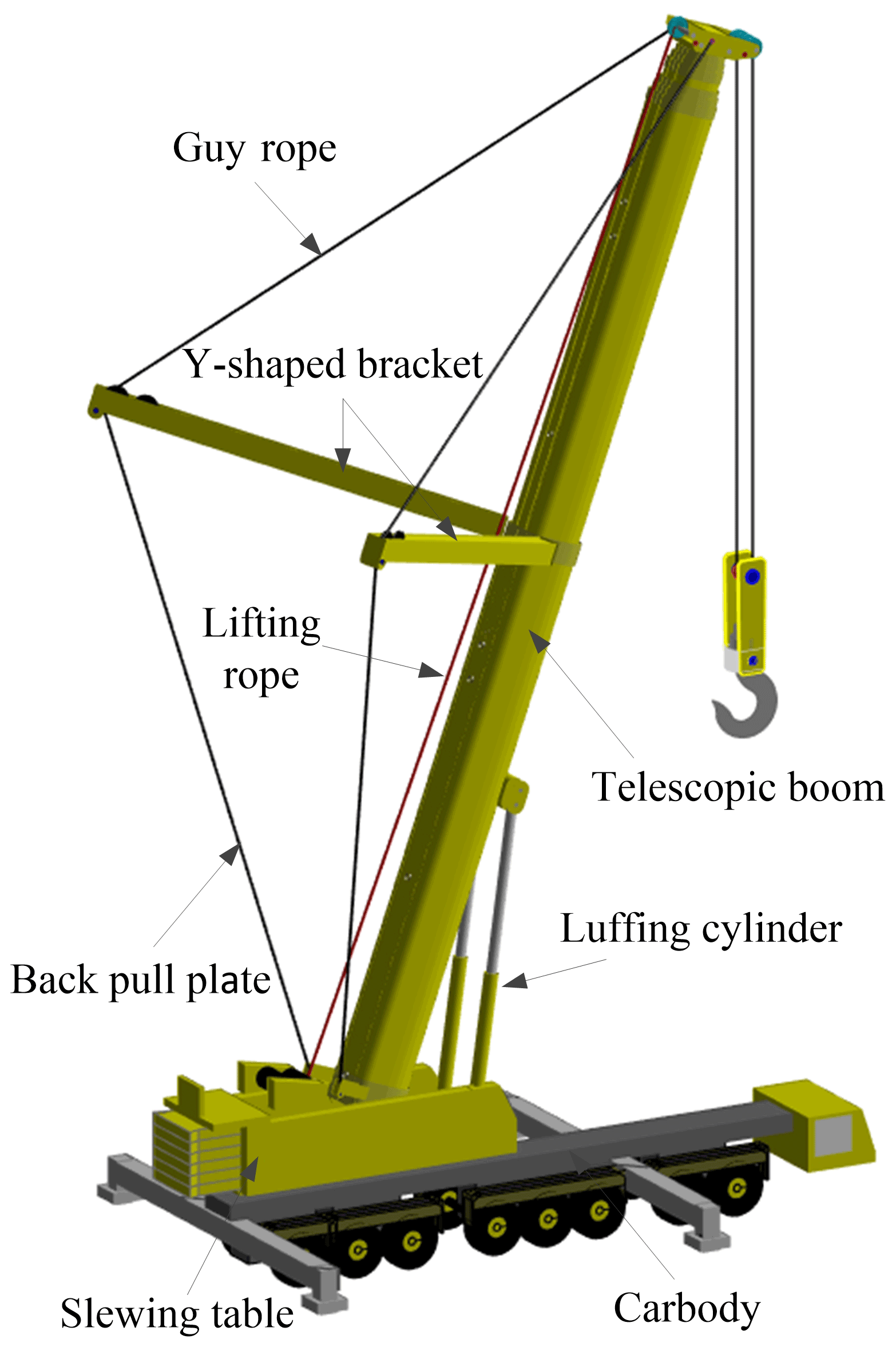
An all-terrain crane is a type of mobile crane. Due to the benefit of its lifting capacity and convenient mobility, it plays an important role in many construction fields (Ja et al., 2019; Yao et al., 2015). The telescopic boom of the all-terrain crane is a typical slender structure composed of multiple boom sections nested in one other. Each boom section is a box-type structure. When the telescopic boom carries a heavy load, its overall deformation exhibits a strong geometrical nonlinear effect. However, the integral stability of the slender structure is poor, which is prone to causing structural instability and result in accidents. The instability of the telescopic boom is one of the important reasons for all-terrain crane accidents (Neitzel et al., 2001). The instability load of the telescopic boom is one of the core indicators that determines the lifting capacity of all-terrain cranes. To improve the structural stability of the telescopic boom, a Y-shaped bracket is used to change its load conditions (Yao et al., 2020). The preload is applied to the telescopic boom through the guy rope to make the telescopic boom produce an initial deformation before lifting and reduces the deformation of telescopic boom during lifting. The Y-shaped bracket, the guy rope, and the back pull plate form the super lift system of the all-terrain crane.
In the structural instability analysis, external loads are commonly considered to be control parameters (Wang et al., 2015). Generally, the equilibrium path of the structures is followed by incremental methods as the control parameters changed. Response points, where tangent stiffness matrices become singular, are useful in the practical engineering applications, since they are related to the structural instability. There are generally two methods to determine the critical point of structural instability, i.e., the direct method and indirect method (Shi, 1996). The direct method is to add constraint equations according to the characteristics of the structure at the critical point (Fujii and Okazawa, 1997; Jari et al., 2012; Ding et al., 2014; Adnan and Mazen, 2000) and then directly solve the critical point based on the Newton–Raphson method. Most direct methods can converge from the region near the critical point to the critical point, and the point in the iterative process is not necessarily on the solution path. Most indirect methods determine whether there is a critical point according to the sign change in the determinant value of the structural tangent stiffness matrix on the structural equilibrium path (Bergan et al., 1978; Shi and Crisfield, 1994). A considerable number of constraint strategies are used to accurately determine the critical load and limit point, including load control, state control, and different kinds of arc length methods (Hellweg and Crisfield, 1998; Lu et al., 2005; Athisakul and Chucheepsakul, 2007). Although these methods have good adaptability in the structural stability calculation, they are also faced with the problem that the step size cannot be adjusted to achieve the required accuracy in the calculation process (Crisfield, 1983).
A correct and effective finite element model must be established for describing the geometrical nonlinear effect of the telescopic boom. At present, three approaches are often used for the finite element analysis of nonlinear solid and structural mechanics, namely total Lagrangian (TL; Pai et al., 2000; Nanakorn and Vu, 2006), updated Lagrangian (UL; Yang et al., 2007; Iu and Bradford, 2010), and co-rotational (CR) formulations (Crisfield and Moita, 1996; Felippa and Haugen, 2005; Li, 2007). Specifically, the CR formulation is suitable for describing the geometric nonlinearity of slender structures whose displacements and rotations may be arbitrarily large, while the local deformations are small. The CR formulations for a stability analysis of beams and shells have been studied by many researchers (Kisu, 1997; Hsiao and Lin, 2000; Battini and Pacoste, 2002; Verlinden et al., 2018).
Since the telescopic boom with a super lift system contains a large number of components, resulting in large-scale degrees of freedom to be solved, the CR formulation is more suitable for a finite element modeling of such slender structures composed of multiple boom sections. The whole structure is divided into several substructures, and the mechanical information of the internal nodes of a single sub structure is condensed to the boundary nodes, including the stiffness matrix (distributed forces), load matrix, etc. This substructure, formed by condensation, is called the super element, which is regarded as an individual element in the whole structural model during the modeling or analysis procedure (Li and Zhao, 2006). The substructure is defined by the characteristic points on a single boom section, and the nodal degrees of freedom in the substructure are statically condensed to form a super element, which reduces the computational burden for solving the global system variables (Mäkinen, 2007; Ghosh and Roy, 2009; He et al., 2010; Rantalainen et al., 2013). The precondition of adopting the static condensation method is that the nodal displacements and rotational angles are small in substructure, and the static condensation must be implemented in local coordinate systems.
The guy rope of the all-terrain crane connects the Y-shaped bracket and the telescopic boom head, which changes the initial deformation of the telescopic boom through a preload. Therefore, the unstressed original length of the guy rope must be calculated with the initial configuration of the telescopic boom without lifting the load, and then nonlinear equilibrium equations of the complete system can be established. Most existing work on cables mainly focuses on calculations with original length and without strain parameters (Jayaraman and Knudson, 1981; Gosling and Korban, 2001; Lee et al., 2003; Ju and Choo, 2005; Wang et al., 2015). However, calculating the unstressed original length of the guy rope under a known preload is necessary for the analysis of all-terrain cranes with super lift system. This calculation method has been studied in previous work (see Xu et al., 2022).
The purpose of this paper, therefore, is to establish the equilibrium equations of telescopic boom of an all-terrain crane, making use of co-rotational formulations, where a static condensation technique for the substructures and the nonlinear external forces from the guy rope with preload are integrated. It needs to be clarified that the material nonlinearity is not considered in this paper. After establishing the nonlinear equilibrium equations with the lifting load containing the control parameter, the accurate tangent stiffness matrix of the equations is derived based on the derivative of the equilibrium equations for the structural displacements. Finally, the load displacement curves of nodes in the telescopic boom are obtained by solving the differential form of the equilibrium equations. Combined with the singularity detection of the tangent stiffness matrix and the judgment criterion, the instability load is obtained.
The key points of this paper are mainly reflected in two aspects. First, the CR formulation is used to calculate the geometric nonlinear effect of the telescopic boom. Compared with the traditional method of establishing the CR formulations on each element (Wempner, 1969; Belytschko and Hsieh, 1973), the static condensation method is used to convert the corresponding substructure into a super element with two nodes, taking into account the influence of the self-weight and the external wind load, which has further improved the traditional static condensation method with zero external load (Przemieniecki, 1963; Bahar and Bahar, 2018). At the same time, the proposed super element can greatly reduce the dimension of the structural equilibrium equations. Second, the traditional load increment method needs to set a fixed load increment in the process of calculating the nonlinear equilibrium equations to obtain the structural equilibrium path (Wang et al., 2017). If the fixed increment is set too small, it will increase the calculation amount and reduce the calculation efficiency (Cheng et al., 1980). If the increment is too large, then the convergence may fail. Moreover, because it is impossible to accurately judge the range of the critical load in advance, the load increment is likely to directly cross the extreme point, which will lead to the failure of searching for the critical load. In this paper, the derivation of lifting the load parameter from the structural equilibrium equations of telescopic boom is converted into differential equations. With the advantage of automatic step size adjustment in the conventional differential equation solver, the function of automatically adjusting the load step size according to the corresponding nonlinearity of the current load state of the system is realized. Under the premise of ensuring the convergence of each step of solution, the structural equilibrium path can be quickly tracked and the critical load can be searched.
This paper takes a certain type of all-terrain crane as an example, as shown in Fig. 1. The telescopic boom is composed of eight boom sections, which can be combined into a boom with a length of 100 m. The combination of different lengths of the telescopic boom can be realized through the telescopic mechanism. The telescopic boom is connected to the slewing table with a shaft, and its luffing angle can be changed by a luffing cylinder. The Y-shaped bracket is installed on the first boom section of the telescopic boom. In accordance with the structural characteristics, the length of each boom is much larger than its section size, and the influence of shear deformation can be ignored. Therefore, a 3D Euler–Bernoulli beam element can be used for the finite element modeling of the telescopic boom. The boom section modulus in tension, bending, and torsion can be illustrated by the user-defined actual parameters of boom section (Dou et al., 2013). Unfortunately, this occurs under the assumption that cross sections of the beam element are rigid. In terms of the telescopic boom, some special conditions in engineering need to be calculated by establishing plate and shell element separately for local verification.
2.1 Division of substructure and local coordinate system
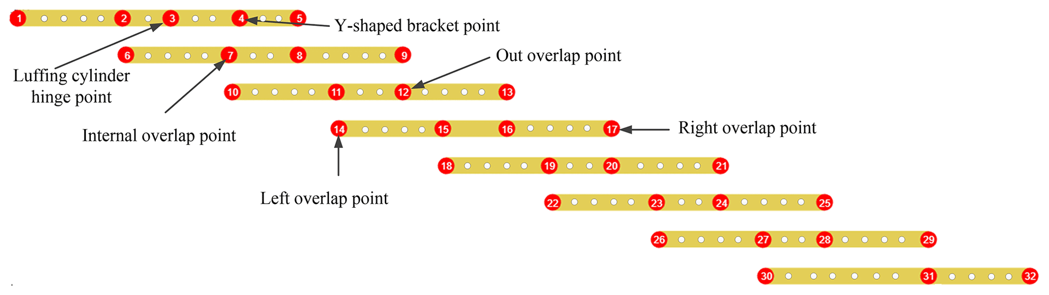
Each boom section is divided into several substructures by the hinge point of the luffing cylinder, Y-shaped bracket, and overlap points between the boom sections, as shown in Fig. 2.
Unfortunately, the static condensation procedure cannot be used directly for the calculation of the geometrical nonlinear analysis of slender structures. However, if a co-rotational formulation for a substructure can be given, in which the elastic displacements and rotational angles are small, then the static condensation technique can be implemented for the telescopic boom structures. A substructure of the boom section after deflection is shown in Fig. 3. Euler angles and Cardan angles are widely used as generalized coordinates to describe the large rotation of the substructure (Wen, 1987; Cekus and Pawel, 2021). Due to the different rotation order of the Euler angle and the Cardan angle, in many practical applications in engineering, the latter is less singular than the former in a numerical calculation. Therefore, this paper uses Cardan angles to establish the transformation matrix between local coordinate system and global coordinate system.
Crisfield and Moita (1996) presented a unified formulation of the co-rotational approach for 3D elements with both translational and rotational degrees of freedom (Battini and Pacoste, 2002; Felippa and Haugen, 2005). The local coordinate system of the substructure is established at one side node of the substructure, and it is described by the global rotational angles (Cardan angles). A single substructure is a generalized beam element composed of multiple initially divided elements, and the origin of its section coordinate system is the node of the generalized beam element. The origin of the section coordinate system is not consistent with the section centroid, as shown in Fig. 3.

are base vectors of the global coordinate system of the telescopic boom system. The position vector of the origin of the substructure in the global coordinate system is r1, and the right endpoint position vector is r2. Global rotational angles are θ1, θ2, which are Cardan angles and can be used to describe the spatial rotation of the substructure coordinate system (Qi, 2008). A transformation matrix between local and global coordinate system is R1. Its column vector can be determined by parameters as follows:
where s1=sin α1, c1=cos α1, s2=sin β1; c2=cos β1, s3=sin γ1, and c3=cos γ1.
is a local coordinate system of a substructure. The position vector and derivative of right endpoint are given by the following:
where is initial position vector of the right node in local coordinate system, and is a translational displacement vector of the right node in local coordinate system. The corresponding virtual velocity is as follows:
where ω1 is the global angular velocity of the left end section. Its conversion relationship with θ1 is as follows:
The virtual velocity of the degree of freedom in the global coordinate system is decomposed into three parts, i.e., the translational virtual velocity, the rotational virtual velocity, and the virtual velocity of the local degree of freedom in a local coordinate system.
The global angular velocity of the right endpoint section is given according to Eq. (4), as follows:
According to the angular velocity superposition principle (Qi, 2008), ω2 can be given with , which is the angular velocity in the local coordinate system, as follows:
In a local coordinate system, the rotation of the section coordinate system is small (Betsch and Steinmann, 2003), combining Eq. (5), as follows:
where is the rotational angle of the right end section of the substructure in a local coordinate system.
The virtual velocity of Eq. (6) is as follows:
The transformation relationship between local and global degrees of freedom needs to be given for transforming the virtual power equations into the following algebraic equation:
where , are local translational displacement vectors in local coordinate system. Their derivatives are as follows:
where a vector with a symbol “∼” on the top is its skew symmetric matrix. For example, if a vector , then its skew symmetric matrix is expressed as follows:
can be obtained according to , which is a rotational matrix of section coordinate system to the local coordinate system, as follows:
According to Eq. (8), its derivative is as follows:
The derivative of a substructure of nodal variables in a global coordinate system is as follows:
Combining Eqs. (10) and (12) yields the following:
The transformation relationship between the variables in local coordinate system and global coordinate system is as follows:
where .
2.2 Eccentric beam element
Each boom section of the telescopic boom is a slender box structure, and its finite element model can be built by 3D Euler–Bernoulli beam element. The nodal parameters of Euler–Bernoulli beam elements are located at the centroid of the section, and its linear stiffness matrix can be written as follows:
where ; ; ; ; ; ; ; . The parameters E, A, Iy, Iz, G, J, and Le are the corresponding Young's modulus, cross-sectional area, y-axis moment of inertia, z-axis moment of inertia, shear modulus, polar moment of inertia, and the length of a beam element.
The section of the telescopic boom section is symmetrical about the y axis and asymmetric about the z axis, so it belongs to a kind of eccentric beam element, as shown in Fig. 3. However, in engineering, the selection of the nodal parameters to reflect the section characteristics is more appropriate, which can avoid the non-coincidence of nodal parameters between nested boom sections. For a single beam element in a substructure, the nodal parameters of the nodes at both ends in the element coordinate system are , . Based on the assumption of a rigid section of the beam element, the rotational angles of its section are consistent, and the rotational angles in the element coordinate system are small. Without losing generality, the position vector of the section centroid in the section coordinate system is . and are displacements at centroid in section coordinate system.
where
The conversion between the nodal parameters at the centroid and the origin of the section coordinate system is as follows:
where
For a beam element, the deformation virtual power of the centroid parameters of the beam element can be transformed into the parameters of the origin of the section coordinate system as follows:
where , . The stiffness matrix of the eccentric beam element is .
2.3 Influence of gravity and wind load of substructure
During the operation of an all-terrain crane, the luffing angle of the telescopic boom changes continuously, so that the influence direction of gravity on the telescopic boom also changes, which cannot meet the condition that the external force of the traditional static condensation method is zero in the internal degree of freedom. The gravity in each element of the substructure is a uniformly distributed force. When the static condensation method is used to condense the structural degrees of freedom, then the self-weight of the element needs to be dispersed to the nodes at both ends.
The position vector of any point in the element of a substructure and its derivative are as follows:
where , are the position vector and displacements of any point in beam element in local coordinate system, R1 is the transformation matrix of the local coordinate system, and ω1 is angular velocity of the local coordinate system.
The rotational angles of any point in the element can be obtained by the interpolation of nodal parameters at both ends for Euler–Bernoulli beam as follows:
where Nu, Nθ are displacements and the rotational angle interpolation shape function of a 3D Euler–Bernoulli beam element (Qi, 2008).
By integrating the length of the beam element, it is seen that the virtual power of gravity has the following substructure:
The resultant force and moment at the origin of the local coordinate system are as follows:
where is the component of the gravitational acceleration g in the global coordinate system, me is the mass of beam element with length Le, and and are position vectors of nodes at both ends of beam element in local coordinate system.
Combing Eqs. (21) and (25) yields the following:
Generalized forces distributed at the nodes at both ends of the element become the following:
The gravity influence coefficient matrix is as follows:
Base on the actual working conditions, the external force on the telescopic boom during operation needs to consider whether the influence of wind load, the factors of the boom section shape, and boom expansion nesting have been considered. A wind load diagram is shown in Fig. 3.
In each substructure, the wind load of each element is equivalently calculated to the origin of the local coordinate system, and the linear density of its resultant force and resultant moment is and . The virtual power of the wind load in the element is as follows:
where the resultant force and moment at the origin of the local coordinate system are
The physical meaning of the generalized force fw distributed at the nodes is as follows:
where , .
The wind load influence coefficient matrix is obtained according to Eqs. (20), (21), (24), and (31) as follows:
2.4 Static condensation of substructure and super element
The local coordinate system is established for a substructure in which the nodal displacements are small. The nodes in each substructure can be divided into two groups, namely internal nodes ni and boundary nodes nb. The gravity and wind load of all elements in the substructure have been converted to the element nodes; therefore, the internal node degrees of freedom of the substructure can be condensed to the boundary node degrees of freedom to form a super element. In the local coordinate system, each beam element stiffness matrix is assembled to form the global stiffness matrix of substructure and is divided into blocks according to the degrees of freedom of boundary nodes and internal nodes.
The deformation virtual power of a substructure can be expressed in a local system as follows:
where and are the boundary and internal nodal degrees of freedom in a substructure.
The total virtual power of gravity and wind load in substructure can be written as follows:
where Gi is the gravity influence coefficient matrix corresponding to the internal node degrees of freedom in the substructure. is the wind load corresponding to the internal node degrees of freedom according to the wind load influence coefficient matrix. F0 and T0 are the resultant force and moment when the gravity and wind load are equivalent to the origin of the local coordinate system. Fb is the gravity and wind load at the boundary node of the substructure.
Since the substructure boundary conditions and external forces are independent of the internal degrees of freedom, is independent, and the coefficients in the virtual power expression are not affected by substructure assembly and external forces. According to the principle of virtual power, combining Eqs. (35) and (36) can yield the following:
Internal degrees of freedom can be written as follows:
The internal nodal displacements in the local coordinate system are small, so the elements in the stiffness matrix are constant, and the virtual velocity of Eq. (38) is
where the incidence matrix is
Substituting Eqs. (39) and (40) into Eqs. (35) and (36) yields the following:
Considering Eqs. (14), (15), and (18), Eqs. (41) and (42) can be written as follows:
The generalized internal and generalized external force are, respectively, written as follows:
The substructure composed of multiple beam elements is reduced to a super beam element expressed by degrees of freedom at both ends, and Ke is its equivalent stiffness matrix.
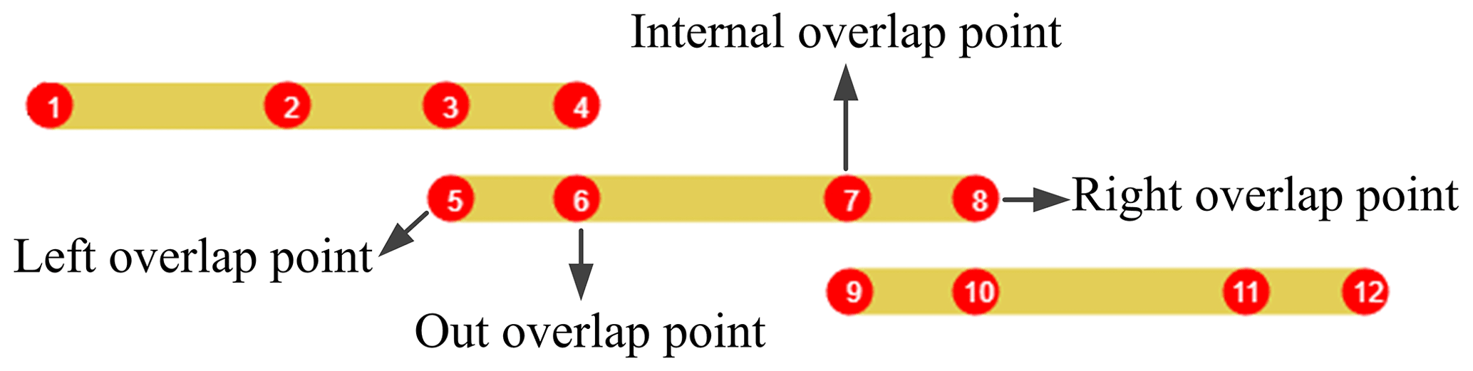
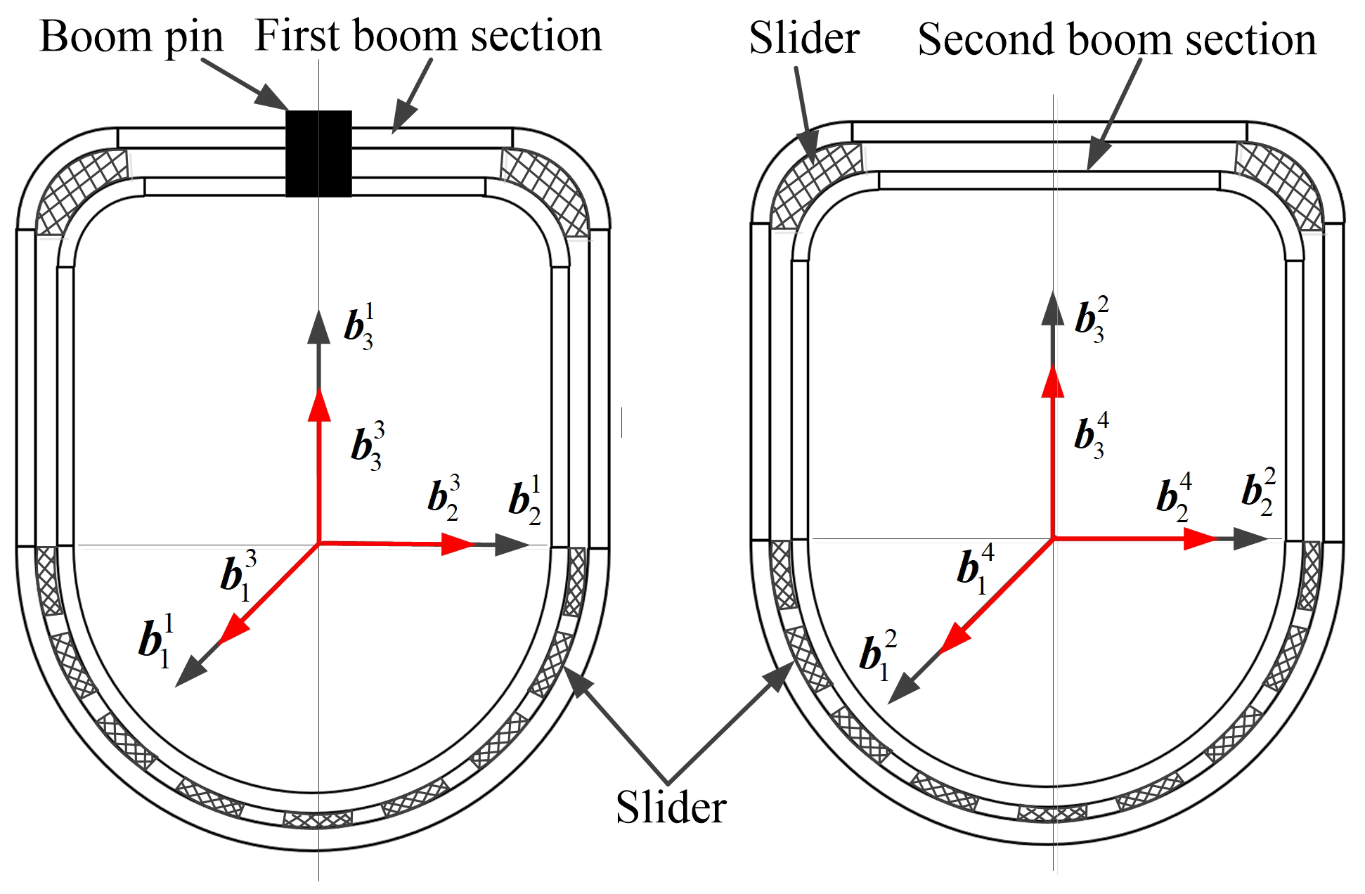
The nested connection of the telescopic boom of an all-terrain crane is the form of a hydraulic cylinder and pin; that is, different combinations of multiple boom sections are realized successively through the telescopic hydraulic cylinder in the first boom section. Each boom section is connected through the boom pin at the tail, and a nylon slider is designed at the tail and head of the boom section for overlapping. Except for the first and last boom sections, four sections in each boom section generate relevant constraints between the outer and inner boom sections. The left overlap point, right overlap point, internal overlap point, and outer overlap point are shown in Fig. 4.
The divided substructure is a super element in each boom section. We take three boom sections as an example, as shown in Fig. 5.
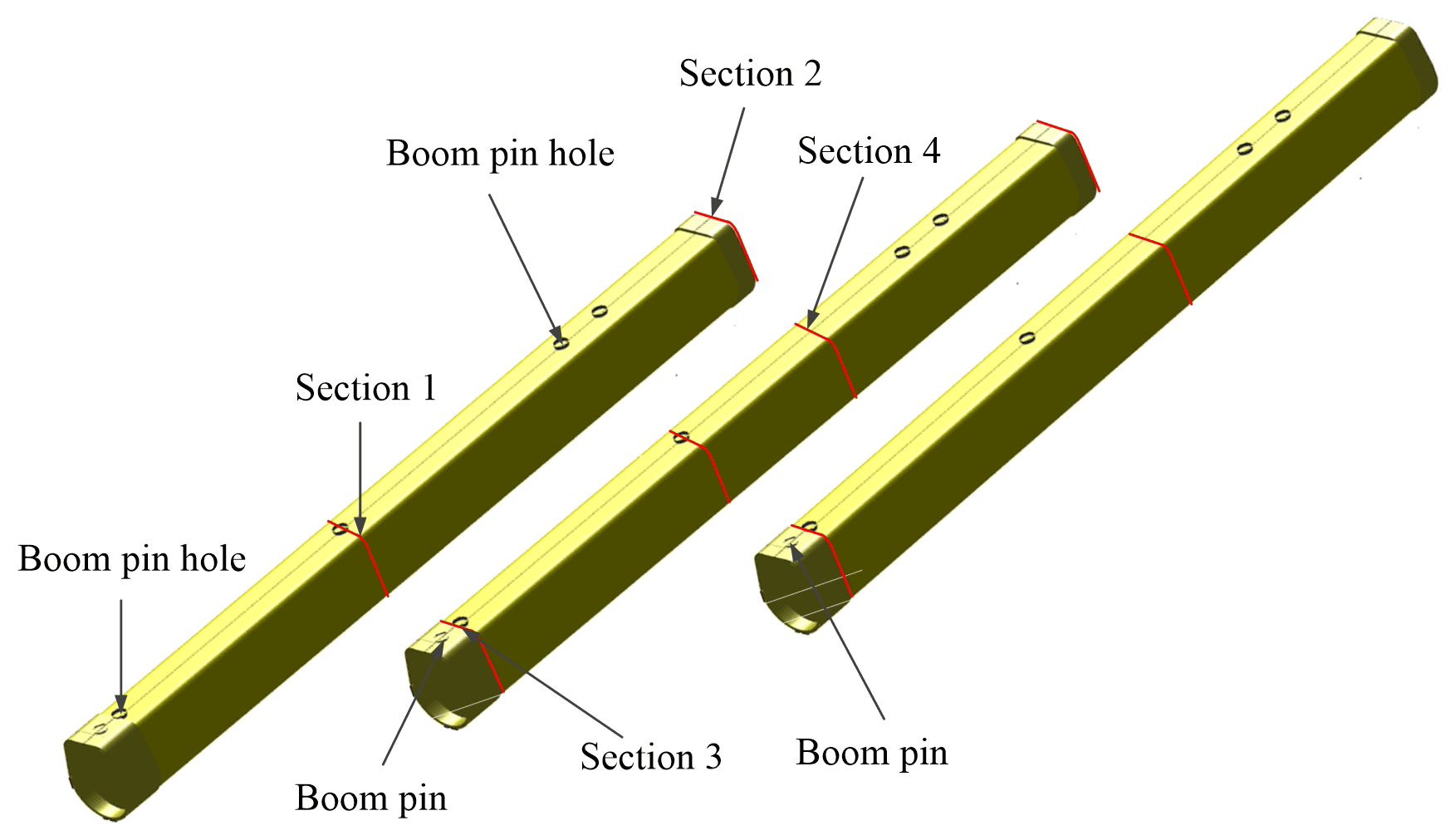
3.1 Constraints between boom sections
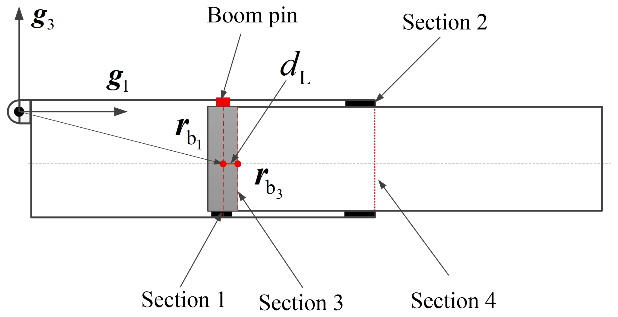
The first two boom sections are used to explain the constraints between them. The connection of the two boom sections corresponds to two types of constraints, where section 1 and section 3 correspond to the rotating joint in the multi-body theory and only have the rotational degrees of freedom about the axis of the boom pin, and section 2 and section 4 correspond to the prismatic joint, which constrains the displacements around the main axis of the section and the rotational degrees of freedom around the normal part of the section. The nodal position vectors and rotational angles in the global coordinate system for the left and right overlap points are , αi, βi, and γi. The corresponding section coordinate system is , which is shown in Fig. 6.
According to the structural form of the boom pin connection, the local part can be regarded as a rigid body. dL is the horizontal distance between the origin of the two local coordinate systems in the initial configuration, as shown in Fig. 7. The constraint equations at the boom pin connection can be written as follows:
The constraint equations at the right end of the first boom section with sliders can be written as follows:
3.2 Boundary constraints of telescopic boom
There is only an independent rotational degree of freedom around the boom foot pin axis, which can be considered to be the boom luffing angle. The local structure can be processed as a rigid part, according to the actual structure at the boom foot, as shown in Fig. 8a.
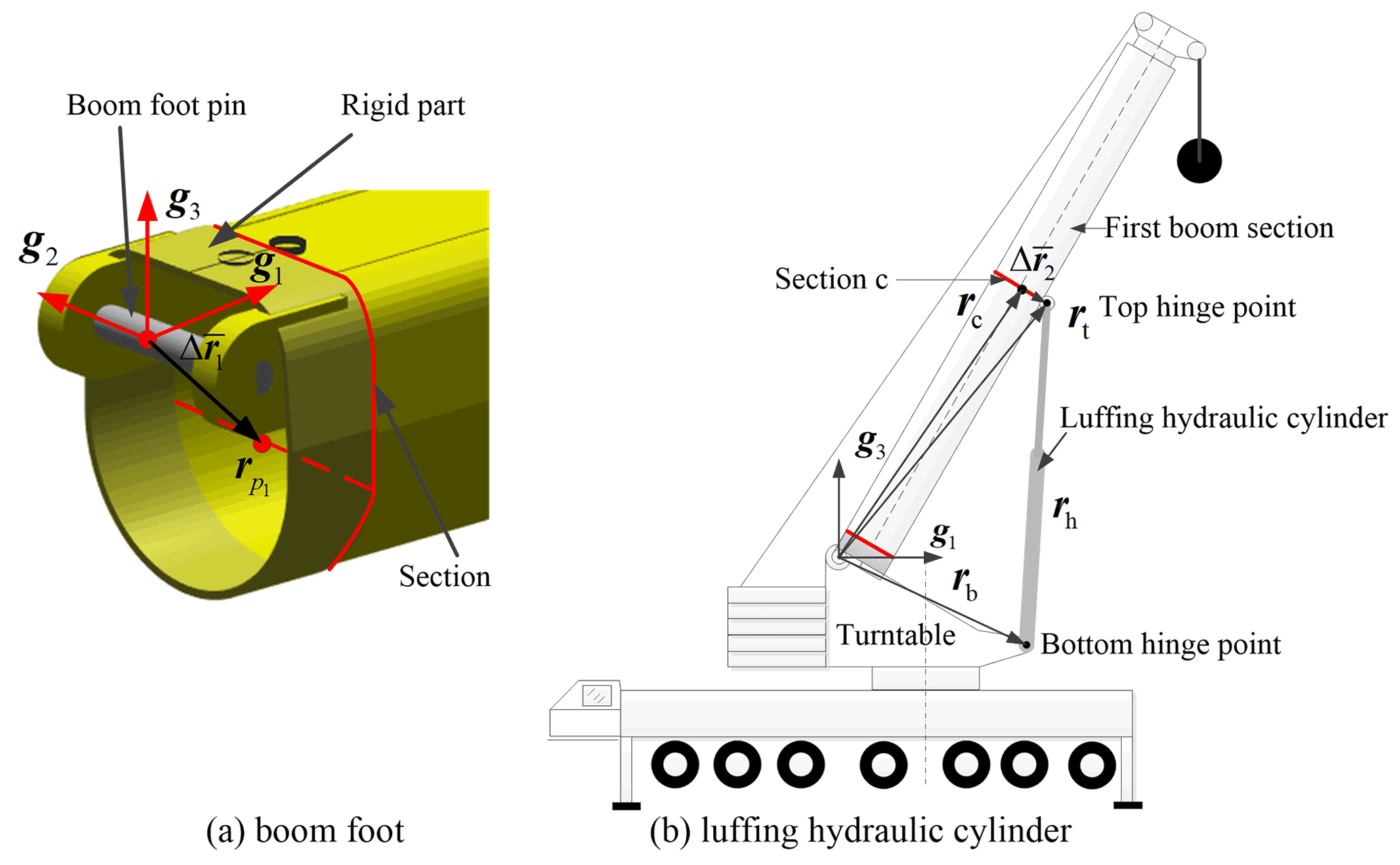
The rigid part has the same angular velocity as the local coordinate system of the first super element. Therefore, the luffing angle degree of freedom can be expressed by the Cardan angle β1 in the global coordinate system. β1 is used as the independent degree of freedom at the constraint of boom foot pin, and the corresponding rotational matrix can be written as follows:
The position vector of the left end node in the global coordinate system is , and the rotational angles are . The constraint equations of the boom foot pin are
The luffing of the telescopic boom is achieved by the luffing hydraulic cylinder, whose bottom and top hinge points are, respectively, connected with the slewing table and the first boom section, as shown in Fig. 8b. The luffing hydraulic cylinder is regarded as a constant length constraint in the finite element modeling and calculation. rc and θc are the nodal variables of top hinge point, and the position vector of top hinge point is as follows:
where Rc is the transformation matrix at top hinge point section, which is formed by the base vectors of the local coordinate system.
The length of the luffing hydraulic cylinder under the corresponding luffing angle is a fixed value, rh is the position vector of the luffing hydraulic cylinder in global coordinate system, and the constraint equation can be written as follows:
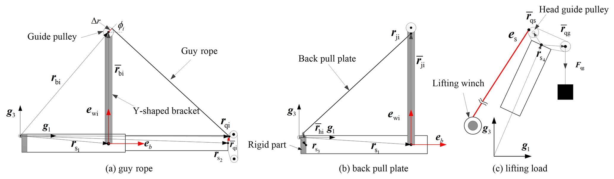
The external nodal forces in the telescopic boom system equations are applied to the nodes of the super element, including the self-weight, external wind load, guy rope force, back pull plate force, and lifting load, as shown in Fig. 9. The first two kind of loads have been considered in Sect. 3. The last two kind of loads can be referred to in a previous work (Xu et al., 2022). A method for calculating the unstressed original length of a guy rope with known preload is derived. After the unstressed original length of the guy rope is obtained by applying the preload under the unloaded state of the telescopic boom, the force of guy rope acting on boom system can be calculated during the lifting process.
4.1 Guy rope force
Base on the structural characteristics of all-terrain crane, the Y-shaped bracket remains perpendicular to the axial direction of the telescopic boom after installation and has good stiffness. It can be considered to be a rigid part in the calculation of the telescopic boom. The Y-shaped bracket and the guy rope are symmetrically connected on both sides.
As shown in Fig. 9a, and are the nodal position vectors and rotational angles of the Y-shaped bracket on the section of the telescopic boom installation point. and are the variables of the node, which is the boom head connecting point. eb and are the unit vectors of the telescopic boom axis and Y-shaped bracket axis, respectively. are the position vectors of the guide pulley in local coordinate system. are the azimuth of the guy rope. A single side guy rope connection is selected for the description.
The derivative of the guide pulley's center in the global coordinate system is as follows:
Here, is the transformation matrix at the Y-shaped bracket installation point section, which is formed by the base vector of the local coordinate system. is the coefficient matrix of the angular velocity of the local coordinate system.
The position vector of the guy rope entry point at the guide pulley and its derivative are as follows:
Here, Δr is the radius of the guide pulley, and .
The position vector of the guy rope connecting point at boom head and its derivative are as follows:
The loads acting on the guide pulley and the connecting point of the guy rope are Fp1, Fp2, Fq1, and Fq2, respectively, which can be calculated on the premise that the original length of the guy rope is known under the corresponding working conditions. The virtual power of the guy rope force to the telescopic boom can be expressed as follows:
4.2 Back pull plate force
The original length of the back pull plate is known, as shown in Fig. 9b. The forces of the plate on the connecting point of the Y-shaped bracket and the first boom section can be calculated with the method in the literature (Xu et al., 2022). Forces on both sides are Fj1, Fj2, Fh1, and Fh2, respectively. and are the nodal position vector and rotational angles of the back pull plate at the connection point. The hinge point at the foot of the boom is fixed axis rotation constraint, and the independent degree of freedom is β3. and are the position vectors of the back pull plate connection point in a local coordinate system.
The derivative of the connection point between back pull plate in a global coordinate system is as follows:
The derivative of a connection point between the back pull plate and foot boom section in global coordinate system is as follows:
The virtual power at the Y-shaped bracket connection point is as follows:
The virtual power at the foot boom section connection point is as follows:
4.3 Lifting load and single lifting rope load
As shown in Fig. 9c, and are the position vectors of the equivalent action point of lifting load and lifting rope in the local coordinate system of a boom head connection. Fqg is the lifting load force under a corresponding working condition. es is the unit vector of the lifting rope between the boom guide pulley and the lifting winch. nq is the number of lifting ropes corresponding to the lifting load, and the single lifting rope force is as follows:
The derivative of a lifting load action point in the global coordinate system is as follows:
The derivative of a lifting rope action point in the global coordinate system is as follows:
The virtual power of a lifting load and the single lifting rope acting on the telescopic boom is as follows:
5.1 System equilibrium equations and tangent stiffness matrix
Taking the degrees of freedom of the boundary nodes in each substructure as system variables and dividing them according to translation and rotation, the global virtual power equations of the telescopic boom can be obtained as follows:
where and are external forces and moments acting on nodes in the global coordinate system. rk0 and θk0 are the position vector and rotational angles of the origin of the kth substructure coordinate system in global coordinate system. Fk0 and Mk0 are the resultant force and moment of gravity and wind load of the kth substructure on its coordinate system origin. and are the equivalent nodal force and moment in the kth substructure coordinate system, which can be expressed as follows:
where the submatrixes , , , and can be obtained from the condensed substructure stiffness matrix Ke. and can be obtained from the gravity influence coefficient matrix Gg. and are the force and moment generated by the wind load condensed to the substructure nodes. and are the displacements and rotational angles of the nodes at both end section origins in the local coordinate system.
According to the transformation relationship between the local and global coordinate system variables in Eq. (18), the transformation matrix of the displacements and the rotational angles of the kth substructure can be transformed into the following:
Equation (66) can be converted into algebraic equations. The virtual power equations of the equivalent nodal forces and moments of the kth substructure can be transformed into the following:
where the degrees of freedom of the kth substructure in the global coordinate system are .
The set of system variables can be defined as q. Combining Eqs. (66) and (70), the global virtual power equations of the telescopic boom can be expressed as follows:
where F(q) is the generalized nodal force matrix of the system.
According to the constraints and boundary conditions between the boom sections of the telescopic boom, the non-independent and independent degrees of freedom in the system variables are divided as .
The constraint equations of the telescopic boom system are established by combining Eqs. (46)–(47), (49), and (51), which include the constraints between the boom sections, the constraints between the telescopic boom and the slewing table, and the constraints between the luffing cylinder. Without losing generality, the constraint equations of the telescopic boom can be expressed as follows:
The variation constraint equations derived from Eq. (72) are obtained as follows:
The virtual variation in the non-independent degrees of freedom can be expressed by independent degrees of freedom, as follows:
Substituting Eq. (74) into Eq. (71), the transformed algebraic equation can be obtained from the following:
After the equations are transformed, the number of equations is the same as the number of independent variables, and the number of non-independent variables is the same as the number of constraint equations added in the system. Combining Eqs. (72) and (75), the system equations for solving the system variables can be obtained as follows:
The above formula is a set of highly nonlinear equations, and the corresponding tangent stiffness matrix is given, which can greatly improve the computational efficiency of the system.
In order to obtain the tangent stiffness matrix of the system equations, the derivative of Eq. (76) can be obtained as follows:
where
Equation (78) is related to the time derivative of the equivalent nodal force and moment in the coordinate system of the kth substructure and the time derivative of the resultant force and moment generated by the gravity and wind load at the origin of the local coordinate system.
Substituting the generalized force matrix F(q) into Eq. (78) yields the following:
where fnd is the corresponding submatrix of the non-independent degrees of freedom in the generalized force matrix F(q).
The time derivative of the constraint equations in Eq. (76) can be obtained as follows:
Substituting Eqs. (78)–(82) into Eq. (77) and combining the results with Eq. (83) above, the tangent stiffness matrix of the system can be obtained.
5.2 Differential form of equilibrium equations and instability load
The instability load of the telescopic boom of all-terrain cranes, especially for the medium and long booms, is a key indicator in the lifting ability. R(q) is obtained by combining Eqs. (57), (60)–(61), and (76), which consists of the guy rope force, the back pull plate force, the generalized node internal force, and system constraint equations. The lifting load is the variable of external force in the system equations, and the related load is in Eq. (65). As shown in Fig. 15, since the lifting load and the single lifting rope load do not directly act on the node when the lifting load is a unit load, the generalized force related to the lifting load can be obtained, i.e., the generalized force matrix G0 corresponding to the unit lifting load. The nonlinear equilibrium equations of the system can be established by R(q) and the generalized force matrix G0 related to the lifting load through the virtual power equations of the assembly system. To sum up, the telescopic boom meets the structural equilibrium under any lifting load, and the nonlinear equilibrium equations of the telescopic boom can be expressed as follows:
where q is the system variable, including nodal displacements and rotational angles of all nodes in the telescopic boom, and λ is the lifting load parameter.
For Eq. (84), in order to obtain the instability load under the systematic consideration of structural nonlinear effects, the conventional method is to divide the load into multiple load steps, through the incremental method, and obtain the corresponding node displacement under each load through calculation, so as to establish the corresponding equilibrium path curve. During the solution process, we monitor the curve slope under all loads, i.e., . Theoretically, when the slope is infinite, then the load corresponding to this extreme point is the critical instability load of the structure. Therefore, it is necessary to set a threshold value as the judgment criterion of the instability load of the telescopic boom system, so as to obtain the instability load.
where K0 is the ratio of the current state parameters to the initial state parameters, i.e., the slope ratio of the equilibrium path curve.
Combined with the above contents, the key point is to obtain the slope of the equilibrium path curve in the process of the changing load, and then determine the instability load in combination with the judgment criterion. In the process of searching for the instability load, the lifting load parameter λ is an unknown variable, and then the derivative of λ in Eq. (84) can be obtained to obtain the corresponding differential equations, as follows:
where is the tangent stiffness matrix of the telescopic boom, which has been obtained in Sect. 5.1. can reflect the nonlinearity of the load displacement curve under the current load.
Furthermore, the first derivative of system variables to the lifting load can be obtained by Eq. (86), as follows:
With the advantage of an automatic step adjustment in ODE113, a conventional differential equation solver of MATLAB, Eq. (87) is solved to realize the function of automatically adjusting the step size according to the nonlinear degree corresponding to the current load state of the system with initial value, λ=0. When the structure is in the linear stage, the solution step can be automatically increased. When the structure is in the nonlinear stage, the step can be automatically reduced. Under the premise of ensuring the convergence of each step of solution, it can quickly track the equilibrium path and search for the instability load. Compared with the traditional incremental method and arc length method, this method can greatly reduce the number of solutions and improve the calculation efficiency.
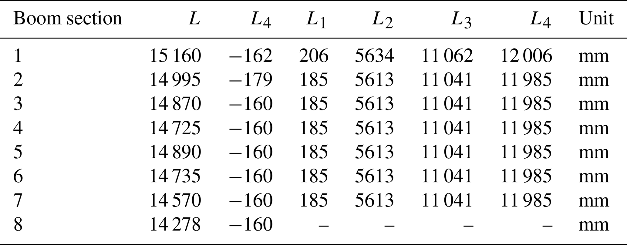


The relevant numerical examples in this section are calculated based on the actual structural parameters of a certain type of all-terrain crane. The Young modulus of elasticity of boom sections material is Pa, material density is kg m−3, and Poisson's ratio is ν=0.3. The telescopic boom is composed of eight boom sections, each boom section contains one boom pin and four pin holes, and their positions along the length of the boom section are recorded as L0, L1, L2, L3, and L4, as shown in Table 1.
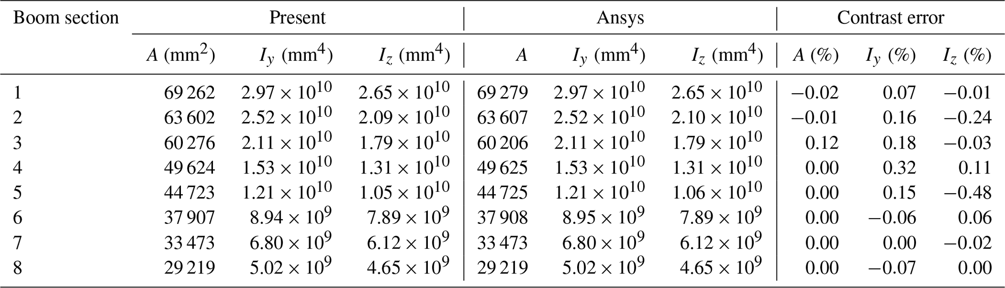
In the commercial software Ansys19.1, the BEAM188 element is used to customize the section according to the section parameters of each boom section, and the section moment of inertia and area are calculated. The section parameters calculated in this paper, and their comparison, are shown in Table 2.
6.1 Example 1 of a cantilever beam about the boom section
In this example, a cantilever beam model is taken as the calculation object for relevant calculation comparison, as shown in Fig. 10. The combination of different lengths of the telescopic boom is realized by different connection modes of the boom pin and the pin hole between boom sections. The super element of the same boom section with different combinations is different. Four connection modes are defined here, corresponding to the lengths of different telescopic boom combinations shown in Fig. 11.
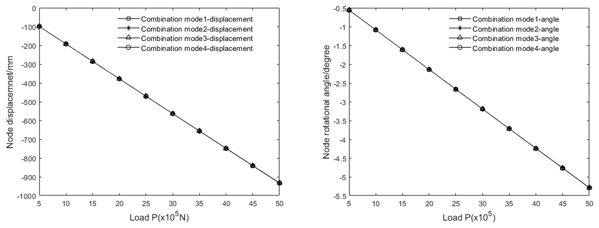
The boom section 1 is taken as calculation model, which is constrained as a cantilever beam. The end load is applied to the origin of the section coordinate system. The z-direction displacement and rotational angle around the y axis of the right end node of four combination modes are calculated under different super elements, as shown in Fig. 11.
Through the comparison of calculation results in Fig. 12, it can be seen that, for the same boom section, when different super elements are used, the error in calculation results is very small, and the calculation results are consistent.
6.2 Example 2 of cantilever beam about boom section
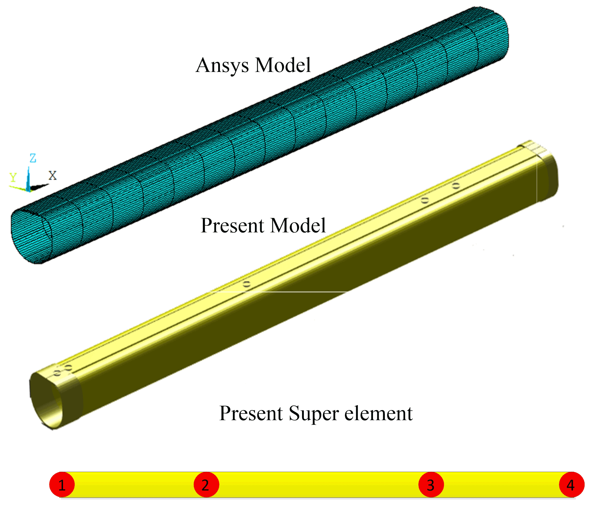
Taking boom section 7 as the calculation model, the division of a super element is established by the combination of mode 3, which is divided into three super elements with a total of 24 degrees of freedom. As shown in Fig. 11, the load application mode and constraint form are established. A model consistent with its section and length parameters is established in the Ansys software, which is divided into 15 elements with a total of 96 degrees of freedom, according to the basic length of the subelement in a super element of this paper. The two model diagrams are shown in Fig. 13.
Different discrete loads are applied at the section centroid of the right end section of the model. Considering the geometrical nonlinear effect of the structure, Ansys software sets the load step as 20 in a large displacement calculation. The vertical z-direction displacements and rotational angles around the y axis of the end nodes of the two models are calculated. The load displacements and rotational angles comparison curves are shown in Fig. 14.
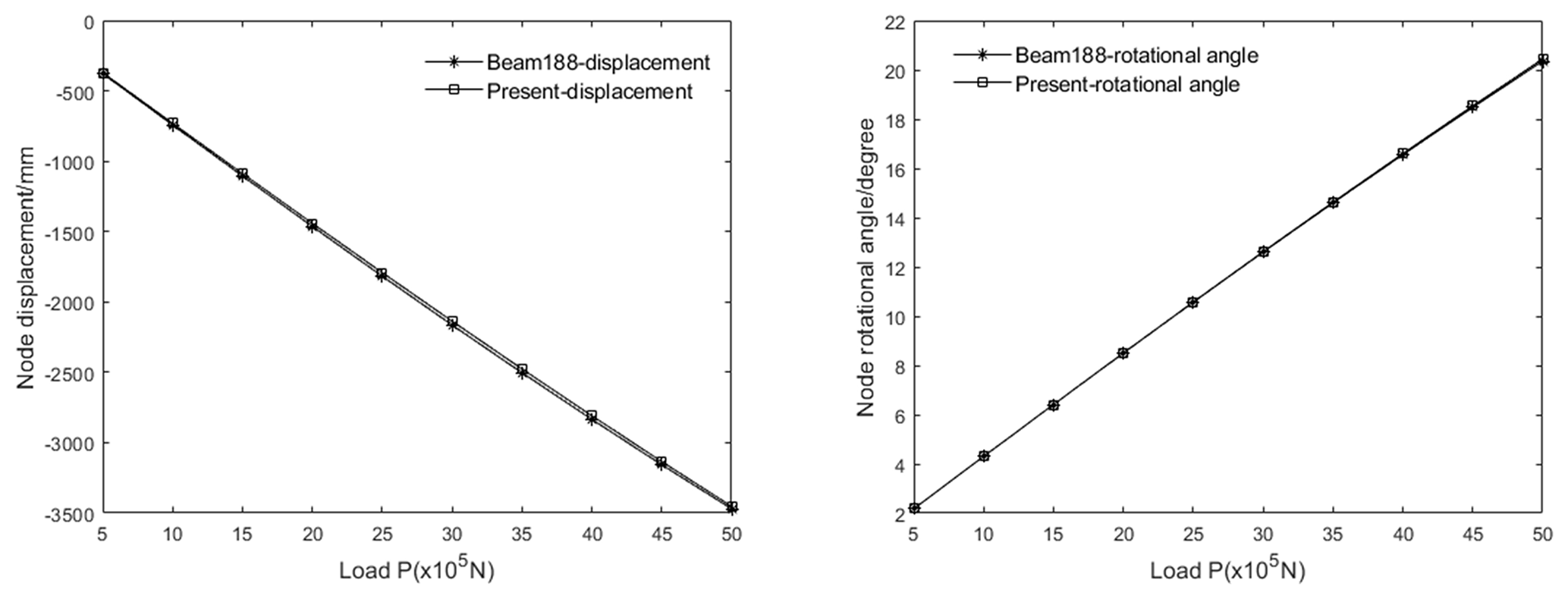
The calculation model is divided into several substructures, the calculation degrees of freedom are reduced by static condensation, and the co-rotational formulation method is used to consider the geometrical nonlinear effect of the whole structure, which improves the efficiency of numerical calculation. At the same time, through a curve comparison, it can be seen that the calculation results obtained by the two different models have small errors, and the errors in the displacements and rotational angles can meet the requirements of the calculation errors in engineering.
6.3 Instability load of the all-terrain crane with a super lift system
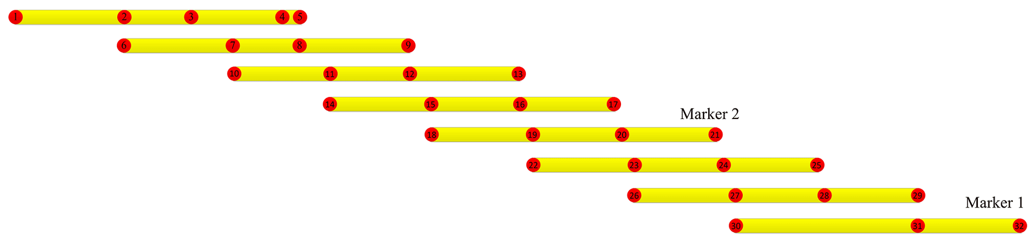
In this example, eight boom sections are assembled into a telescopic boom, with the length being 55.5 m in accordance with connection mode 2. The node number of the telescopic boom is shown in Fig. 15. The preload of the guy rope is applied on the telescopic boom to resist the deformation of self-weight before lifting the load. From the engineering point of view, the larger the initial luffing angle of the telescopic boom, the smaller the preload of the guy rope to overcome the deformation will be. In this example, the luffing angle of the telescopic boom is 83∘.
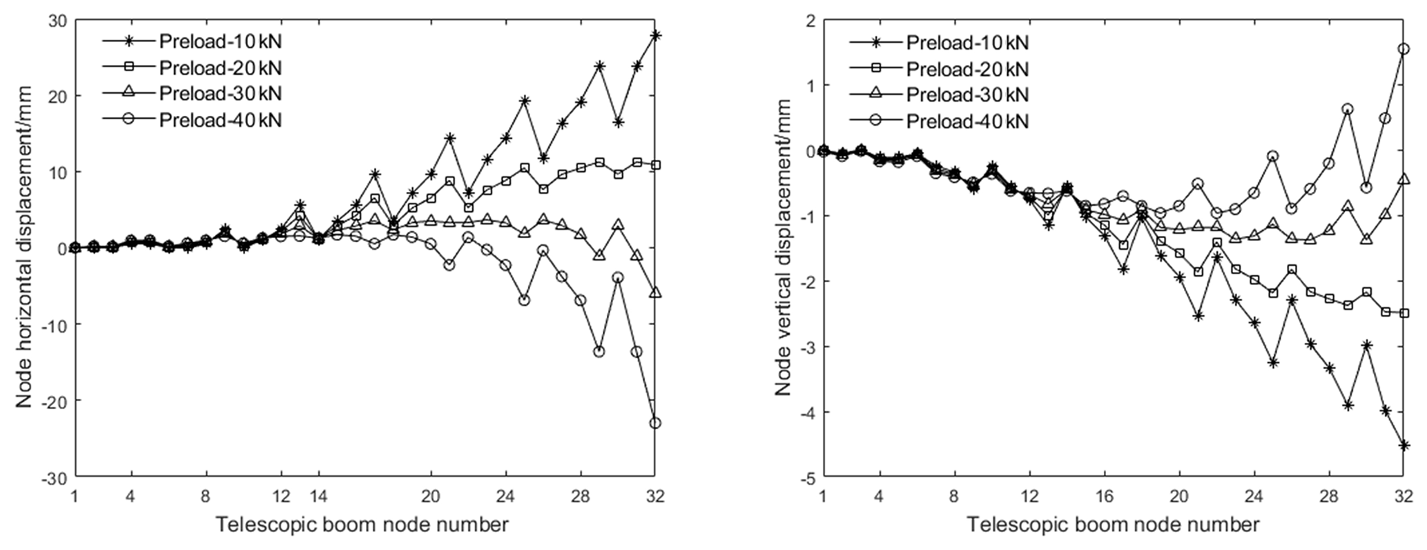
The preload is discretized from 10 to 40 kN into four preloads for application, and the nodal displacements of the telescopic boom relative to the horizontal and vertical directions of the initial position under different preload conditions are obtained, as shown in Fig. 16.
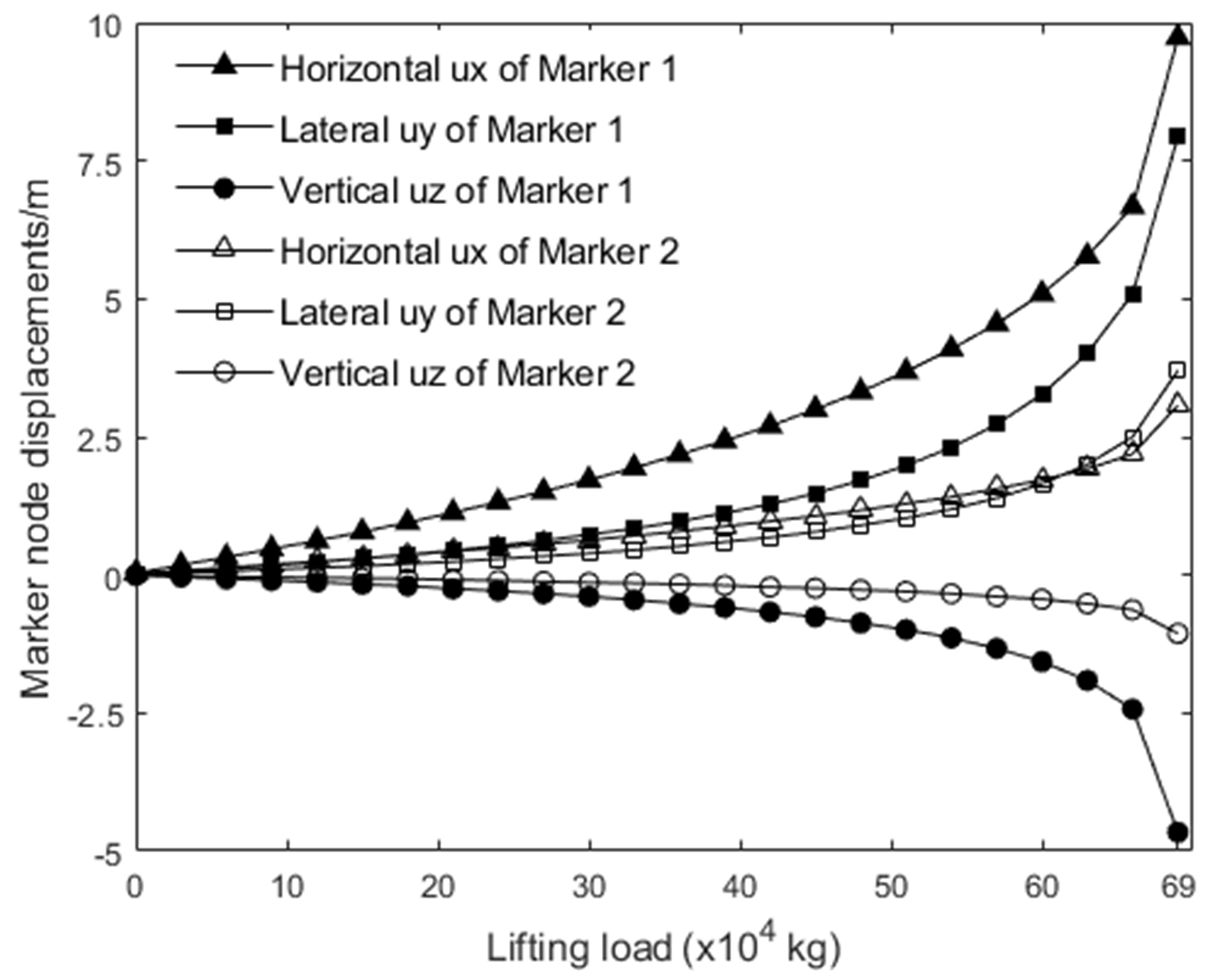
Combining with the engineering practice, taking 20 kN as the preload of the guy rope, the original length of the guy rope is calculated, and the subsequent calculation is carried out on this basis. In Fig. 15, the displacements of marker 1 and marker 2 points change with the increasing load, and the final load displacement curves are shown in Fig. 17. It can be seen from the curve that the lifting load is 6.9×10⁵ kg, and the slope of the load displacement curve increases sharply at that point, which can be considered to be the critical instability load of the telescopic boom.
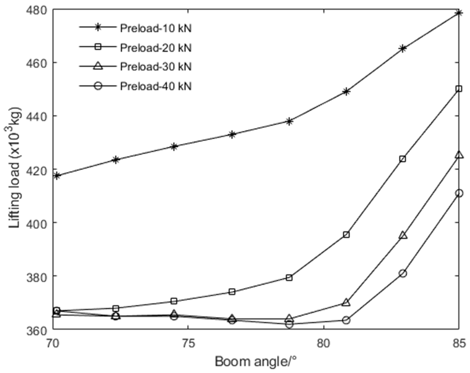
In practical engineering, the critical instability load cannot be used as the rated load of the all-terrain crane. During the calculation, we monitor the slope change in the load displacement curve of marker 1 and marker 2 points and take the ratio of the real-time slope to the initial slope as the judgment criterion, which is 3 in this calculation example. The most reasonable value of this criterion needs to be selected through a large number of calculations and tests. The instability load curve of the telescopic boom with different preloads, and the range of luffing angle at 70 to 85∘, is shown in Fig. 18.
It can be seen from Fig. 18 that, with the increase in preload in the initial state, the deformation of telescopic boom in the initial state is reduced to a certain extent, and even the reverse bending deformation appears. At the same time, the axial load of the telescopic boom increases, and the instability load shows a downward trend in Fig. 18. For the lifting capacity determined by the whole telescopic boom, it also includes the load determined by the structural strength of the boom. The final lifting capacity is data determined by comprehensive factors, and the structural strength load will be studied in follow-up research.
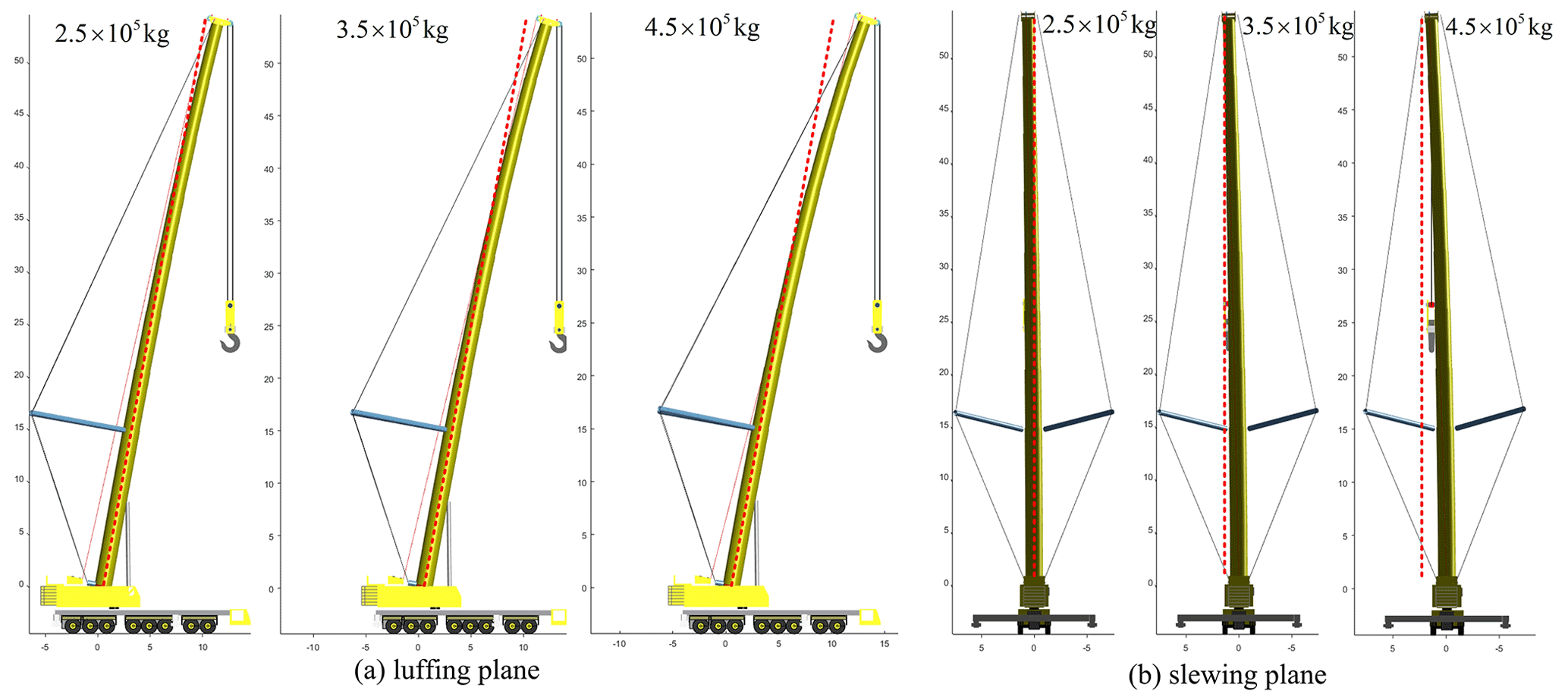
The preload of guy rope is 20 kN, and three lifting loads are selected for calculation, with the lateral load ratio being 3 % of the lifting load, which acts on the boom head. The deformations in the luffing plane and slewing plane are shown in Fig. 19.
The instability load of the telescopic boom of an all-terrain crane can be obtained based on the differential form of system governing equations. First, for each boom section, the corresponding substructure is established by selecting reasonable boundary nodes, and the internal degrees of freedom of the substructure are reduced by static condensation method to form a super element. The approximately specific beam relationship between the corresponding boom sections and the boundary conditions of the telescopic boom are given. Second, based on the proposed geometrical nonlinear calculation method of the cable element, the nonlinear external force at the guy rope connection node of the telescopic boom with initial preload is presented. The equilibrium equations of telescopic boom with the control parameters of load are derived based on co-rotational procedures, and the tangent stiffness of the equilibrium equations are formulated. Finally, the equilibrium equations are transformed into differential form, and the load displacement curves are illustrated by solving the differential equations with existing numerical methods. A method to calculate the structural equilibrium path and instability load of the telescopic boom of the all-terrain crane with a guy rope preload is given, which provides a certain theoretical support for the design of the all-terrain crane.
| Base vectors of the global coordinate system for telescopic boom | |
| Base vectors of the local coordinate system for a substructure | |
| g | Gravity acceleration in global coordinate system |
| r1,r2 | Current global position vectors of the two end-section origins of a substructure |
| θ1,θ2 | Global rotational angles of the two end-sections of a substructure (Cardan angles) |
| Initial position vectors of the two end-section origins for a substructure in local coordinate system | |
| Translational displacement vectors of the two end-section origins for a substructure in local coordinate system | |
| ω1,ω2 | Global angular velocities of the two end-sections of a substructure |
| Angular velocities in local coordinate system of a right section of a substructure | |
| Rotational angle vectors of two end-sections of a substructure in a local coordinate system | |
| R1,R2 | Global rotational matrices of the two end-sections of a substructure |
| Transformation matrix between a right section and a local coordinate system of a substructure | |
| Local displacement vectors of the two section origins of a beam element in beam coordinate system | |
| Local translational displacement vectors of the two-section centroid of a beam element in a beam coordinate system | |
| Local rotational angle vectors of the two end-sections of a beam element in a beam coordinate system | |
| Element stiffness matrix based on a section centroid and section origin parameters | |
| Ke | Stiffness matrix of a super element |
| Current global and initial local position vectors of any point in a beam element | |
| me,Le | Mass per unit length and length of a beam element |
| Gg | Gravity influence coefficient matrix |
| G1,G2 | Wind load influence coefficient matrix |
| Base vectors of the local coordinate system of a boom section |
| Overlap point angular velocities coefficient matrix of boom section overlap point | |
| Telescopic boom, Y-shaped bracket, and lifting rope axial base vectors | |
| q | Telescopic boom system variables with independent and dependent variables |
| Γid | Transformation matrix between independent variables and system variables |
| Φ(q) | Constraint equations of the telescopic boom system |
| G0 | Generalized force matrix corresponding to the unit lifting load |
| λ | Lifting load parameter |
The code and processed data required to reproduce these findings cannot be shared at this time, as the data also form part of an ongoing study.
JX was responsible for writing the paper and the mechanical equipment model. YZ and TZ developed part of the software. ZQ developed the methodology and software. GW checked the procedure, and TW calculated the examples.
The contact author has declared that none of the authors has any competing interests.
Publisher's note: Copernicus Publications remains neutral with regard to jurisdictional claims in published maps and institutional affiliations.
This research has been supported by the Foundation for Innovative Research Groups of the National Natural Science Foundation of China (grant nos. 11872137, 11802048, and 91748203).
This paper was edited by Engin Tanık and reviewed by two anonymous referees.
Adnan, I. and Mazen, A. M.: Quadratically convergent direct calculation of critical points for 3d structures undergoing finite rotations, Comput. Method Appl. M., 189, 107–120, https://doi.org/10.1016/S0045-7825(99)00291-1, 2000.
Athisakul, C. and Chucheepsakul, S.: Effect of inclination on bending of variable-arc-length beams subjected to uniform self-weight, Eng. Struct., 30, 902–908, https://doi.org/10.1016/j.engstruct.2007.04.010, 2007.
Bahar, H. and Bahar, A.: A force analogy method (FAM) assessment on different static condensation procedures for frames with full rayleigh damping, Struct. Des. Tall Spec., 27, E1468, https://doi.org/10.1002/tal.1468, 2018.
Bergan, P. G., Horrigmoe, G., Krakeland, B., and Soreide, T. H.: Solution techniques for non-linear finite element problems, Int. J. Numer. Meth. Eng., 12, 1677–1696, https://doi.org/10.1002/nme.1620121106, 1978.
Battini, J. M. and Pacoste, C.: Co-rotational beam elements with warping effects in instability problems, Comput. Method Appl. M., 191, 1755–1789, https://doi.org/10.1016/S0045-7825(01)00352-8, 2002.
Belytschko T. and Hsieh B. J.: Non-linear transient finite element analysis with convected co-ordinates, Int. J. Numer. Meth. Eng., 7, 255–271, https://doi.org/10.1002/nme.1620070304, 1973.
Betsch, P. and Steinmann, P.: Constrained dynamics of geometrically exact beams, Comput. Mech., 31, 49–59, https://doi.org/10.1016/j.cma.2005.05.002, 2003.
Cekus, D. and Paweł, K.: Method of determining the effective surface area of a rigid body under wind disturbances, Arch. Appl. Mech., 91, 1–14, https://doi.org/10.1007/s00419-020-01753-9, 2021.
Cheng, S. Y., Hsu, T. R., and Too, J. J. M.: An integrated load increment method for finite elasto-plastic stress analysis, Int. J. Numer. Meth. Eng., 15, 833–842, https://doi.org/10.1002/nme.1620150604, 1980.
Crisfield, M. A.: An arc-length method including line searches and accelerations, Int. J. Nume. Meth. in Eng., 19, 1269–1289, https://doi.org/10.1002/nme.1620190902, 1983.
Crisfield, M. A. and Moita, G. F.: A unified co-rotational framework for solids, shells and beams, Int. J. Solids. Struct., 33, 2969–2992, https://doi.org/10.1016/0020-7683(95)00252-9, 1996.
Dou, C., Guo, Y. L., Zhao, S. Y., Pi, Y. L., and Bradford M. A.: Elastic out-of-plane buckling load of circular steel tubular truss arches incorporating shearing effects, Eng. Struct., 52, 697–706, https://doi.org/10.1016/j.engstruct.2013.03.030, 2013.
Ding, J. Y., Wallin, M., Cheng, W., Recuero, A. M., and Shabana, A. A.: Use of independent rotation field in the large displacement analysis of beams, Nonlinear Dynam., 76, 1829–1843, https://doi.org/10.1007/s11071-014-1252-1, 2014.
Fujii, F., and Okazawa, S.: Pinpointing bifurcation points and branch-switching, J. Eng. Mech., 123, 179–189, https://doi.org/10.1061/(ASCE)0733-9399(1997)123:3(179), 1997.
Felippa, C. A. and Haugen, B.: A unified formulation of small-strain co-rotational finite elements: I. Theory, Comput. Method Appl. M., 194, 2285–2335, https://doi.org/10.1016/j.cma.2004.07.035, 2005.
Gosling, P. D. and Korban, E. A.: A bendable finite element for the analysis of flexible cable structures, Finite Elem. Anal. Des., 38, 45–63, https://doi.org/10.1016/S0168-874X(01)00049-X, 2001.
Ghosh, S. and Roy, D.: A frame-invariant scheme for the geometrically exact beam using rotation vector parametrization, Comput. Mech., 44, 103–118, https://doi.org/10.1007/s00466-008-0358-z, 2009.
Hellweg, H. B. and Crisfield, M. A.: A new arc-length method for handling sharp snap-backs, Comput. Struct. 66, 705–709, https://doi.org/10.1016/S0045-7949(97)00077-1, 1998.
Hsiao, K. M. and Lin, W. Y.: A co-rotational finite element formulation for buckling and post buckling analyses of spatial beams, Comput. Method Appl. M., 188, 567–594, https://doi.org/10.1016/S0045-7825(99)00284-4, 2000.
He, Y. J., Zhou, X. H., and Hou, P. F.: Combined method of super element and substructure for analysis of ILTDBS reticulated mega-structure with single-layer latticed shell substructures, Finite Elem. Anal. Des., 46, 563–570, https://doi.org/10.1016/j.finel.2010.02.004, 2010.
Iu, C. K. and Bradford, M. A.: Second-order elastic finite element analysis of steel structures using a single element per member, Eng. Struct., 32, 2606–2016, https://doi.org/10.1016/j.engstruct.2010.04.033, 2010.
Jari, M., Reijo, K., Alexis, F., and Heikki, M.: Direct computation of critical equilibrium states for spatial beams and frames, Int. J. Numer. Meth. Eng., 89, 135–153, https://doi.org/10.1002/nme.3233, 2012.
Ja, H. S., Kwang, S. O., and Hong, J. N.: Model predictive control–based steering control algorithm for steering efficiency of a human driver in all-terrain cranes, Adv. Mech. Eng., 11, 1–16, https://doi.org/10.1177/1687814019859783, 2019.
Jayaraman, H. B. and Knudson, W. C.: A curved element for the analysis of cable structures, Comput. Struct., 14, 325–333, https://doi.org/10.1016/0045-7949(81)90016-X, 1981.
Ju, F. and Choo, Y. S.: Super element approach to cable passing through multiple pulleys, Int. J. Solids Struct., 42, 3533–3547, https://doi.org/10.1016/j.ijsolstr.2004.10.014, 2005.
Kisu, L.: Analysis of large displacements and large rotations of three-dimensional beams by using small strains and unit vectors, Commun. Numer. Meth. En., 13, 987–997, 1997.
Lee, K. H., Choo, Y. S., and Ju, F.: Finite element modelling of frictional slip in heavy lift sling systems, Comput. Struct., 81, 2673–2690, https://doi.org/10.1016/S0045-7949(03)00333-X, 2003.
Li, J. and Zhao, X.: A super-element approach for structural identification in time domain, Front. Mech. Eng., 1, 215–221, https://doi.org/10.1007/s11465-006-0004-4, 2006.
Li, Z. X.: A co-rotational formulation for 3D beam element using vectorial rotational variables, Comput. Mech., 39, 309–322, https://doi.org/10.1007/s00466-006-0029-x, 2007.
Lu, M., Schultz, A. E., and Stolarski, H. K.: Application of the arc-length method for the stability analysis of solid unreinforced masonry walls under lateral loads, Eng. Struct., 27, 909–919, https://doi.org/10.1016/j.engstruct.2004.11.018, 2005.
Mäkinen, J.: Total Lagrangian reissner's geometrically exact beam element without singularities, Int. J. Numer. Meth. Eng., 70, 1009–1048, https://doi.org/10.1002/nme.1892, 2007.
Neitzel, R. L., Seixas, N. S., and Ren, K. K.: A review of crane safety in the construction industry, App. OEH., 16, 1106–1117, https://doi.org/10.1080/10473220127411, 2001.
Nanakorn, P. and Vu, L. N.: A 2D field-consistent beam element for large displacement analysis using the total Lagrangian formulation, Finite Elem. Ana. Des., 42, 1240–1247, https://doi.org/10.1016/j.finel.2006.06.002, 2006.
Pai, P. F., Anderson, T. J., and Wheater, E. A.: Large-deformation tests and total-Lagrangian finite-element analyses of flexible beams, Int. J. Solids Struct., 37, 2951–2980, https://doi.org/10.1016/S0020-7683(99)00115-8, 2000.
Przemieniecki, J. S.: Matrix structural analysis of substructures, AIAA J., 1, 138–147, https://doi.org/10.2514/3.1483, 1963.
Qi, Z. H.: Science Press, Dynamics of multibody systems, Beijing, China, ISBN 978-7-03-022473-6, 2008.
Rantalainen, T. T., Mikkola, A. M., and Björk, T. J.: Sub-modeling approach for obtaining structural stress histories during dynamic analysis, Mech. Sci., 4, 21–31, https://doi.org/10.5194/ms-4-21-2013, 2013.
Shi, J.: Computing critical points and secondary paths in nonlinear structural stability analysis by the finite element method, Comput. Struct., 58, 203–220, https://doi.org/10.1016/0045-7949(95)00114-V, 1996.
Shi, J. and Crisfield, M. A.: A semi-direct approach for the computation of singular points, Comput. Struct., 51, 107–115, https://doi.org/10.1016/0045-7949(94)90040-X, 1994.
Verlinden, O., Huynh, H. N., Kouroussis, G., and Rivière-Lorphèvre, E.: Modelling of flexible bodies with minimal coordinates by means of the corotational formulation, Multibody Syst. Dyn., 42, 495–514, https://doi.org/10.1007/s11044-017-9609-0, 2018.
Wang, G., Qi, Z. H., and Kong, X. C.: Geometrical nonlinear and stability analysis for slender frame structures of crawler cranes, Eng. Struct., 83, 209–222, https://doi.org/10.1016/j.engstruct.2014.11.003, 2015.
Wang, W., Duan, Z. Y., and Geng, J. Z.: Geometrically nonlinear structural modeling of large flexible wing based on CR theory, Acta Aeron. Astron. Sin., 38, 88–96, https://doi.org/10.7527/S1000-6893.2017.721544, 2017.
Wempner, G.: Finite elements, finite rotations and small strains of flexible shells, Int. J. Solids Struct., 5, 117–153, https://doi.org/10.1016/0020-7683(69)90025-0, 1969.
Wen, W. F.: Quaternion and relative Euler parameter, J. Jilin Univ., 4, 19–25, https://doi.org/10.13229/j.cnki.jdxbgxb1987.04.025, 1987.
Xu, J. S., Qi, Z. H., Zhuo, Y. P., Zhao, T. J., and Teng, R. M.: A geometric nonlinear calculation method for spatial suspension cable, J. Mech. Eng., 58, 147–156, 2022.
Yang, Y. B., Lin, S. P., and Leu L. J.: Solution strategy and rigid element for nonlinear analysis of elastically structures based on updated Lagrangian formulation, Eng. Struct., 29, 1189–1200, https://doi.org/10.1016/j.engstruct.2006.08.015, 2007.
Yao, J., Qiu, X. M., Zhou, Z. P., Fu, Y. Q., Xing, F., and Zhao, E. F.: Buckling failure analysis of all-terrain crane telescopic boom section, Eng. Fail. Anal., 57, 105–117, https://doi.org/10.1016/j.engfailanal.2015.07.038, 2015.
Yao, F. L., Meng, W. J., Zhao, J., Shi, G. S., Bai, Y. Q., and Li, H.: The relationship between eccentric structure and super-lift device of all-terrain crane based on the overall stability, J. Mech. Sci. Technol., 34, 2365–2370, https://doi.org/10.1007/s12206-020-0513-9, 2020.
- Abstract
- Introduction
- Substructure of telescopic boom and static condensation procedure
- Constraints and boundary conditions of telescopic boom
- External force of the telescopic boom
- Calculation of the instability load
- Numerical examples
- Conclusion
- Appendix A: Nomenclature
- Code and data availability
- Author contributions
- Competing interests
- Disclaimer
- Financial support
- Review statement
- References