Kinematics decoupling analysis of a hyper-redundant manipulator driven by cables

The mapping relationship between the driving space and the workspace is essential for the precise control of a cable-driven hyper-redundant robot. For a hyper-redundant robot driven by cables, the relationships between the driving space and the joint space and between the joint space and the workspace were studied. A joint-decoupling kinematics analysis method was proposed and a kinematic analysis was presented. Based on the analysis of the coupling effect between the cable-driving space and the joint space, a decoupling analysis of the whole cable-driving space and joint space was conducted to eliminate the coupling effect between the joints, and the mapping relationship between the driving cables and the joint angles was obtained. Given the initial and target orientations of the hyper-redundant robot, the variation law for each joint angle was obtained using quintic polynomial trajectory planning and the pseudo-inverse Jacobian matrix, and then the driving cable variation law could be solved. Based on the results, the joint angle changes and the workspace trajectories were solved in turn. By comparing with the initial trajectory, the simulation results verified the appropriateness of the decoupling analysis.

1 Introduction

Hyper-redundant manipulators are highly flexible, so they have significant potential for use in complex spatial operations, such as can be found in the aerospace, aviation, shipbuilding, nuclear power, and emergency rescue fields. Since hyper-redundant manipulators have many degrees of freedom and complex structures, they are difficult to control. If the motor is placed on the mechanical arm, the overall motion's inertia will largely be caused by the weight of the components (Robert et al., 2014). A flexible cable drive can be used to place the driving component in the base so the machine will be lighter and its operation will be more flexible in complex and narrow spaces. Super-redundant manipulators driven by flexible cables have high-precision requirements for the flexible cables' control, and actuated cables with different joints will produce coupling effects during movement (Wang et al., 2017). Therefore, it was necessary to study analytical methods for joint decoupling to eliminate this coupling effect.

In this study, a decoupling analysis for each joint in a hyper-redundant manipulator was conducted, the coupling effect was eliminated for the front joint near the back joint's base, and a mapping relationship between the drive cable and the joint angle was obtained. Since the determination of the unique mapping relationship is the key factor affecting a hyper-redundant manipulator's motion accuracy and control accuracy (Jiang et al., 2020), it is of great importance to analyze the kinematics of the hyper-redundant manipulator's joint angles and drive cables.

2 Mapping relationship between the cable drive and robot kinematics

The forward kinematics solution for robots can construct the mapping relationship between the joint space and the end workspace. The mapping relationship between the flexible drive space and the joint space should be further developed to build the mapping relationship from the flexible drive space to the workspace for a super-redundant manipulator driven by flexible cables. The inverse kinematics between the Cartesian end workspace and the drive space can also be obtained (Bamdad et al., 2019; Yuan et al., 2017; Lamine et al., 2016).

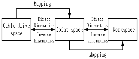
Figure 1 Mapping relationship of the workspace for a hyper-redundant manipulator driven by cables.

Figure 1 shows that the kinematics and mapping relationship for a hyper-redundant manipulator could be divided into two parts. The mapping relationship between the cable drive space and the joint space could be used to obtain the relationship between the joint angle and the cable drive length. Based on the mapping relationship between the robot joint space and the working space, the relationship between the joint angle and the length of the flexible cable could be obtained (Hu et al., 2010).

2.1 Kinematics analyses of the cable drive space and the joint space

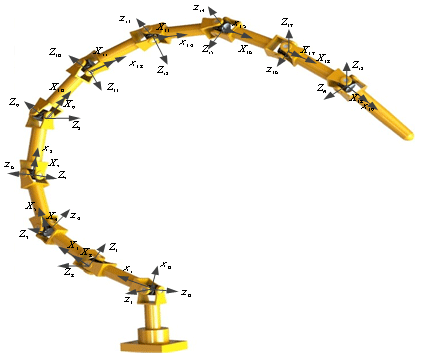
Figure 2 shows that each linkage of a hyper-redundant manipulator was connected by 10 universal joints, and each joint had two degrees of freedom. To facilitate the kinematics analyses, 10 universal joints were divided into 20 equivalent orthogonal joints, and a Denavit–Hartenberg (DH) coordinate system was established. A coordinate system was established at each joint and each coordinate system connected with the frame's coordinate system, no. 0, which was in the direction normal to the frame. The joints' coordinate systems were numbered using sequential integers, beginning with 1. In the 19th coordinate system, the origin of each coordinate system was the joint's point of rotation. The x axis of each bar coordinate system was placed along the bar, and the z axis was set as the drive axis. Finally, the direction of the y axis was determined according to the right-hand rule. By establishing the DH coordinate system, the DH parameters, and the coordinate system transformation matrix, the robot kinematics model was developed.

Figure 2 Kinematics model for a hyper-redundant manipulator.

The homogeneous transformation matrix for each of the hyper-redundant manipulator's coordinate systems was obtained from the kinematics model. The transformation matrix for the end-effector on the base of the hyper-redundant manipulator was obtained by multiplying all of the connecting linkages' transformation matrices to obtain the position and attitude of the end-effector. Since the hyper-redundant manipulator was driven by flexible cables, the joints' rotation angles were determined by variations in the flexible cables' lengths. Therefore, it was necessary to analyze the kinematics of the flexible cables' driving space and joint space.

The kinematics analysis of the cable drive space and the joint space involved determining the corresponding relationship between the joints' rotation angles and driving soft cables' length changes. This was done by building a kinematics model, which described the excessive changes in the joint angle with changes in the driving soft cable length. The relationship between the drive space and the joint space was obtained using an inverse kinematics solution (Mu et al., 2020).

Based on this relationship and the actual task requirements, the end-effector's target position in the workspace was determined. The inverse solution for the hyper-redundant manipulator was obtained from this position, and it was used to determine each joint's rotation angle. The joints' rotation angles could be controlled by adjusting the variations in the flexible cables, enabling the end-effector of the hyper-redundant manipulator to reach the target point (Xu et al., 2017; Zaplana et al., 2018).

Figure 3 Joint of a hyper-redundant manipulator.

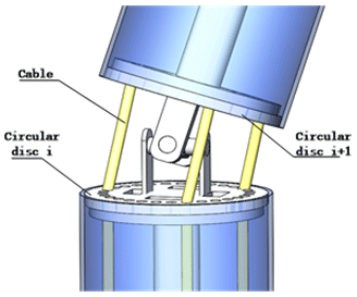
Figure 3 shows that a single joint in the hyper-redundant manipulator had three driven flexible cable inputs and two rotational degree of freedom (DOF) outputs and that this joint was equivalent to a parallel mechanism (Cui et al., 2019). The joint was driven by three independent flexible cables that could obtain two rotational degrees of freedom, so that the hyper-redundant manipulator could move in three-dimensional space. The three cables refer to those installed at joint i in particular. The three cables did not affect the movements of the other joints behind joint i but primarily controlled the change in the rotation angle for this joint.

The lengths of the flexible cables in the linkages did not change while the hyper-redundant manipulator was moving, so the changes in the joint angles were caused by changes in the lengths of the flexible cables between the holes corresponding to the disks at both ends of the joints (Xu et al., 2020). The mapping relationship between the lengths of the flexible cables and the angle of a joint was obtained by analyzing the length changes in the flexible cables during the rotation of each joint and eliminating the cables' coupling influence between different joints.

2.2 Mapping relationship between the cable length and the joint angle

As shown in Fig. 4, plane $A_i^{\mathrm{1}}{A}_i^{\mathrm{2}}{A}_i^{\mathrm{3}}$ and plane $B_{i+\mathrm{1}}^{\mathrm{1}}{B}_{i+\mathrm{1}}^{\mathrm{2}}{B}_{i+\mathrm{1}}^{\mathrm{3}}$ represent disk i and disk i+1, respectively. Line segments $A_i^{\mathrm{1}}{B}_{i+\mathrm{1}}^{\mathrm{1}}$, $A_i^{\mathrm{2}}{B}_{i+\mathrm{1}}^{\mathrm{2}}$, and $A_i^{\mathrm{3}}{B}_{i+\mathrm{1}}^{\mathrm{3}}$ represent the lengths of the joint's three independent cables, and point Q is the center point of the joint. With the centers o_i and o_i+1 on surfaces $A_i^{\mathrm{1}}{A}_i^{\mathrm{2}}{A}_i^{\mathrm{3}}$ and $B_{i+\mathrm{1}}^{\mathrm{1}}{B}_{i+\mathrm{1}}^{\mathrm{2}}{B}_{i+\mathrm{1}}^{\mathrm{3}}$ as the origins, the axial directions of the linkages as the z axes, and the rotational directions of the joint as the x and y axes, the coordinate systems {i} and {i+1} were constructed. As shown in Fig. 2, the central point, Q, of the joint was fixed. For further study and analysis, an intermediate coordinate system, {j}, was constructed at Q.

Figure 4 Analysis of the joint model's coordinate systems.

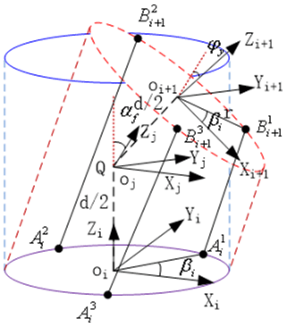
Figure 4 shows that the distance between the joint's two disks in the initial orientation was set as d, and the relationship between the coordinate systems {i} and {j} was determined through translation and a rotation transformation. When the coordinate system {i} was shifted upward by a distance of $d/\mathrm{2}$ and then rotated through an angle of α_f around the x_j axis that coincided with the coordinate system {j}, the homogeneous transformation matrix from the coordinate system {i} to the coordinate system {j} could be obtained. This transformation matrix is expressed in Eq. (1):

$$\begin{array}{}\text{(1)}& \begin{array}{rl}{}_j^{i}T& =\mathrm{Trans}(\mathrm{0},\mathrm{0},d/\mathrm{2})\mathrm{Rot}(X,{\mathit{\alpha }}_f)\\ & =\left[\begin{array}{llll}\mathrm{1}& \mathrm{0}& \mathrm{0}& \mathrm{0}\\ \mathrm{0}& \mathrm{1}& \mathrm{0}& \mathrm{0}\\ \mathrm{0}& \mathrm{0}& \mathrm{1}& d/\mathrm{2}\\ \mathrm{0}& \mathrm{0}& \mathrm{0}& \mathrm{1}\end{array}\right]\left[\begin{array}{llll}\mathrm{1}& \mathrm{0}& \mathrm{0}& \mathrm{0}\\ \mathrm{0}& c{\mathit{\alpha }}_f& -s{\mathit{\alpha }}_f& \mathrm{0}\\ \mathrm{0}& s{\mathit{\alpha }}_f& c{\mathit{\alpha }}_f& \mathrm{0}\\ \mathrm{0}& \mathrm{0}& \mathrm{0}& \mathrm{1}\end{array}\right]\\ & =\left[\begin{array}{llll}\mathrm{1}& \mathrm{0}& \mathrm{0}& \mathrm{0}\\ \mathrm{0}& c{\mathit{\alpha }}_f& -s{\mathit{\alpha }}_f& \mathrm{0}\\ \mathrm{0}& s{\mathit{\alpha }}_f& c{\mathit{\alpha }}_f& d/\mathrm{2}\\ \mathrm{0}& \mathrm{0}& \mathrm{0}& \mathrm{1}\end{array}\right].\end{array}\end{array}$$

The coordinate system {j} rotated through an angle ψ_y around its y axis and then moved a distance of $d/\mathrm{2}$ upward along the z axis of the rotated coordinate system to achieve coincidence with the coordinate system {i+1}. Thus, the transformation matrix from the coordinate system {j} to the coordinate system {i+1} was obtained, as expressed in Eq. (2):

$$\begin{array}{}\text{(2)}& \begin{array}{rl}{}_{i+\mathrm{1}}^{j}T& =\mathrm{Rot}(Y,{\mathit{\psi }}_y)\mathrm{Trans}(\mathrm{0},\mathrm{0},d/\mathrm{2})\\ & =\left[\begin{array}{llll}c{\mathit{\psi }}_y& \mathrm{0}& s{\mathit{\psi }}_y& \mathrm{0}\\ \mathrm{0}& \mathrm{1}& \mathrm{0}& \mathrm{0}\\ -s{\mathit{\psi }}_y& \mathrm{0}& c{\mathit{\psi }}_y& \mathrm{0}\\ \mathrm{0}& \mathrm{0}& \mathrm{0}& \mathrm{1}\end{array}\right]\left[\begin{array}{llll}\mathrm{1}& \mathrm{0}& \mathrm{0}& \mathrm{0}\\ \mathrm{0}& \mathrm{1}& \mathrm{0}& \mathrm{0}\\ \mathrm{0}& \mathrm{0}& \mathrm{1}& d/\mathrm{2}\\ \mathrm{0}& \mathrm{0}& \mathrm{0}& \mathrm{1}\end{array}\right]\\ & =\left[\begin{array}{llll}c{\mathit{\psi }}_y& \mathrm{0}& s{\mathit{\psi }}_y& ds{\mathit{\psi }}_y/\mathrm{2}\\ \mathrm{0}& \mathrm{1}& \mathrm{0}& \mathrm{0}\\ -s{\mathit{\psi }}_y& \mathrm{0}& c{\mathit{\psi }}_y& dc{\mathit{\psi }}_y/\mathrm{2}\\ \mathrm{0}& \mathrm{0}& \mathrm{0}& \mathrm{1}\end{array}\right].\end{array}\end{array}$$

Then the transformation matrix between the coordinate systems {i} and {i+1} was obtained, as shown in Eq. (3):

$$\begin{array}{}\text{(3)}& \begin{array}{rl}{}_{i+\mathrm{1}}^{i}T& ={}_j^{i}T{}_{i+\mathrm{1}}^{j}T\\ & =\left[\begin{array}{llll}\mathrm{1}& \mathrm{0}& \mathrm{0}& \mathrm{0}\\ \mathrm{0}& c{\mathit{\alpha }}_f& -s{\mathit{\alpha }}_f& \mathrm{0}\\ \mathrm{0}& s{\mathit{\alpha }}_f& c{\mathit{\alpha }}_f& d/\mathrm{2}\\ \mathrm{0}& \mathrm{0}& \mathrm{0}& \mathrm{1}\end{array}\right]\left[\begin{array}{llll}c{\mathit{\psi }}_y& \mathrm{0}& s{\mathit{\psi }}_y& ds{\mathit{\psi }}_y/\mathrm{2}\\ \mathrm{0}& \mathrm{1}& \mathrm{0}& \mathrm{0}\\ -s{\mathit{\psi }}_y& \mathrm{0}& c{\mathit{\psi }}_y& c{\mathit{\psi }}_{y}d/\mathrm{2}\\ \mathrm{0}& \mathrm{0}& \mathrm{0}& \mathrm{1}\end{array}\right]\\ & =\left[\begin{array}{llll}c{\mathit{\psi }}_y& \mathrm{0}& s{\mathit{\psi }}_y& s{\mathit{\psi }}_{y}d/\mathrm{2}\\ s{\mathit{\alpha }}_{f}s{\mathit{\psi }}_y,& c{\mathit{\alpha }}_f& -c{\mathit{\psi }}_{y}s{\mathit{\alpha }}_f& -c{\mathit{\psi }}_{y}s{\mathit{\alpha }}_{f}d/\mathrm{2}\\ -c{\mathit{\alpha }}_{f}s{\mathit{\psi }}_y& s{\mathit{\alpha }}_f& c{\mathit{\alpha }}_{f}c{\mathit{\psi }}_y& d/\mathrm{2}+c{\mathit{\alpha }}_{f}c{\mathit{\psi }}_{y}d/\mathrm{2}\\ \mathrm{0}& \mathrm{0}& \mathrm{0}& \mathrm{1}\end{array}\right].\end{array}\end{array}$$

The coordinates of point $B_{i+\mathrm{1}}^{\mathrm{1}}$ in the coordinate system {i} are represented by $(M,N,Q)$, and the coordinates of point $A_i^{\mathrm{1}}$ in the coordinate system {i} are represented by $(m,n,q)$. For point $B_{i+\mathrm{1}}^{\mathrm{1}}$ on disk i+1 with radius r, $\mathrm{\angle }{B}_{i+\mathrm{1}}^{\mathrm{1}}{O}_{i+\mathrm{1}}{X}_{i+\mathrm{1}}={\mathit{\beta }}_i$ could be obtained from Fig. 4. Similarly, point $B_{i+\mathrm{1}}^{\mathrm{1}}$ also corresponded to a point $A_i^{\mathrm{1}}$ on disk i, and $\mathrm{\angle }{A}_i^{\mathrm{1}}{O}_i{X}_i={\mathit{\beta }}_i$ could also be obtained. Thus, the coordinates of point $A_i^{\mathrm{1}}$ in the coordinate system {i} could be expressed as $(m,n,q)=(rc{\mathit{\beta }}_i,rs{\mathit{\beta }}_i,\mathrm{0})$, and the matrix of point $B_{i+\mathrm{1}}^{\mathrm{1}}$ in the coordinate system {i+1} could be expressed as ${}^{i+\mathrm{1}}{B}_{i+\mathrm{1}}^{\mathrm{1}}={\left[\begin{array}{llll}rc{\mathit{\beta }}_i& rs{\mathit{\beta }}_i& \mathrm{0}& \mathrm{1}\end{array}\right]}^T$. Then point $B_{i+\mathrm{1}}^{\mathrm{1}}$ could be expressed as matrix ${}^i{B}_{i+\mathrm{1}}^{\mathrm{1}}$ in the coordinate system {i}, as shown in Eq. (4):

$$\begin{array}{}\text{(4)}& \begin{array}{rl}{}^i{B}_{i+\mathrm{1}}^{\mathrm{1}}& ={}_{i+\mathrm{1}}^{i}T{}^{i+\mathrm{1}}{B}_{i+\mathrm{1}}^{\mathrm{1}}\\ & =\left[\begin{array}{llll}c{\mathit{\psi }}_y& \mathrm{0}& s{\mathit{\psi }}_y& s{\mathit{\psi }}_{y}d/\mathrm{2}\\ s{\mathit{\alpha }}_{f}s{\mathit{\psi }}_y,& c{\mathit{\alpha }}_f& -c{\mathit{\psi }}_{y}s{\mathit{\alpha }}_f& -c{\mathit{\psi }}_{y}s{\mathit{\alpha }}_{f}d/\mathrm{2}\\ -c{\mathit{\alpha }}_{f}s{\mathit{\psi }}_y& s{\mathit{\alpha }}_f& c{\mathit{\alpha }}_{f}c{\mathit{\psi }}_y& d/\mathrm{2}+c{\mathit{\alpha }}_{f}c{\mathit{\psi }}_{y}d/\mathrm{2}\\ \mathrm{0}& \mathrm{0}& \mathrm{0}& \mathrm{1}\end{array}\right]\left[\begin{array}{l}rc{\mathit{\beta }}_i\\ rs{\mathit{\beta }}_i\\ \mathrm{0}\\ \mathrm{1}\end{array}\right]\\ & =\left[\begin{array}{l}s{\mathit{\psi }}_{y}d/\mathrm{2}+rc{\mathit{\psi }}_{y}c{\mathit{\beta }}_i\\ rc{\mathit{\alpha }}_{f}s{\mathit{\beta }}_i-c{\mathit{\psi }}_{y}s{\mathit{\alpha }}_{f}d/\mathrm{2}+\mathrm{rc}{\mathit{\beta }}_{i}s{\mathit{\alpha }}_{f}s{\mathit{\psi }}_y\\ d/\mathrm{2}+c{\mathit{\alpha }}_{f}c{\mathit{\psi }}_{y}d/\mathrm{2}+rs{\mathit{\alpha }}_{f}s{\mathit{\beta }}_i-rc{\mathit{\alpha }}_{f}c{\mathit{\beta }}_{i}s{\mathit{\psi }}_y\\ \mathrm{1}\end{array}\right].\end{array}\end{array}$$

The coordinates of point $B_{i+\mathrm{1}}^{\mathrm{1}}$ in the coordinate system {i} were also obtained and are presented in Eq. (5):

$$\begin{array}{}\text{(5)}& \begin{array}{rl}(M,N,P)& =(s{\mathit{\psi }}_{y}d/\mathrm{2}+rc{\mathit{\psi }}_{y}c{\mathit{\beta }}_i,rc{\mathit{\alpha }}_{f}s{\mathit{\beta }}_i\\ & +rc{\mathit{\beta }}_{i}s{\mathit{\alpha }}_{f}s{\mathit{\psi }}_y-c{\mathit{\psi }}_{y}s{\mathit{\alpha }}_{f}d/\mathrm{2},d/\mathrm{2}\\ & +c{\mathit{\alpha }}_{f}c{\mathit{\psi }}_{y}d/\mathrm{2}+rs{\mathit{\alpha }}_{f}s{\mathit{\beta }}_i-rc{\mathit{\alpha }}_{f}c{\mathit{\beta }}_{i}s{\mathit{\psi }}_y).\end{array}\end{array}$$

Then the length of cable $\left|{}^i{A}_i^{\mathrm{1}}{}^i{B}_{i+\mathrm{1}}^{\mathrm{1}}\right|$ could be expressed by Eq. (6):

$$\begin{array}{}\text{(6)}& \begin{array}{rl}\left|{}^i{A}_i^{\mathrm{1}}{}^i{B}_{i+\mathrm{1}}^{\mathrm{1}}\right|& =\sqrt{(M-m{)}^{\mathrm{2}}+(N-n{)}^{\mathrm{2}}+(P-n{)}^{\mathrm{2}}}\\ & =\left(\right(s{\mathit{\psi }}_{y}d/\mathrm{2}+rc{\mathit{\beta }}_{i}c{\mathit{\psi }}_y-rc{\mathit{\beta }}_i{)}^{\mathrm{2}}\\ & +(rc{\mathit{\alpha }}_{f}s{\mathit{\beta }}_i+rc{\mathit{\beta }}_{i}s{\mathit{\alpha }}_{f}s{\mathit{\psi }}_y-c{\mathit{\psi }}_{y}s{\mathit{\alpha }}_{f}d/\mathrm{2}\\ & -rs{\mathit{\beta }}_i{)}^{\mathrm{2}}+(d/\mathrm{2}+c{\mathit{\alpha }}_{f}c{\mathit{\psi }}_{y}d/\mathrm{2}+rs{\mathit{\alpha }}_{f}s{\mathit{\beta }}_i\\ & -rc{\mathit{\alpha }}_{f}c{\mathit{\beta }}_{i}s{\mathit{\psi }}_y{)}^{\mathrm{2}}{)}^{\mathrm{1}/\mathrm{2}}.\end{array}\end{array}$$

Similarly, Eqs. (7) and (8) describe the lengths of cables $\left|{}^i{A}_i^{\mathrm{2}}{}^i{B}_{i+\mathrm{1}}^{\mathrm{2}}\right|$ and $\left|{}^i{A}_i^{\mathrm{3}}{}^i{B}_{i+\mathrm{1}}^{\mathrm{3}}\right|$, respectively:

$$\begin{array}{}\text{(7)}& {\displaystyle }\begin{array}{rl}\left|{}^i{A}_i^{\mathrm{2}}{}^i{B}_{i+\mathrm{1}}^{\mathrm{2}}\right|& =\left(\right(s{\mathit{\psi }}_{y}d/\mathrm{2}+rc{\mathit{\beta }}_{i+\mathrm{2}\mathit{\pi }/\mathrm{3}}c{\mathit{\psi }}_y-rc{\mathit{\beta }}_{i+\mathrm{2}\mathit{\pi }/\mathrm{3}}{)}^{\mathrm{2}}\\ & +(rc{\mathit{\alpha }}_{f}s{\mathit{\beta }}_{i+\mathrm{2}\mathit{\pi }/\mathrm{3}}+rc{\mathit{\beta }}_{i+\mathrm{2}\mathit{\pi }/\mathrm{3}}s{\mathit{\alpha }}_{f}s{\mathit{\psi }}_y\\ & -c{\mathit{\psi }}_{y}s{\mathit{\alpha }}_{f}d/\mathrm{2}-rs{\mathit{\beta }}_{i+\mathrm{2}\mathit{\pi }/\mathrm{3}}{)}^{\mathrm{2}}\\ & +(d/\mathrm{2}+c{\mathit{\alpha }}_{f}c{\mathit{\psi }}_{y}d/\mathrm{2}+rs{\mathit{\alpha }}_{f}s{\mathit{\beta }}_{i+\mathrm{2}\mathit{\pi }/\mathrm{3}}\\ & -rc{\mathit{\alpha }}_{f}c{\mathit{\beta }}_{i+\mathrm{2}\mathit{\pi }/\mathrm{3}}s{\mathit{\psi }}_y{)}^{\mathrm{2}}{)}^{\mathrm{1}/\mathrm{2}},\end{array}\text{(8)}& {\displaystyle }\begin{array}{rl}\left|{}^i{A}_i^{\mathrm{3}}{}^i{B}_{i+\mathrm{1}}^{\mathrm{3}}\right|& =\left(\right(s{\mathit{\psi }}_{y}d/\mathrm{2}+rc{\mathit{\beta }}_{i+\mathrm{4}\mathit{\pi }/\mathrm{3}}c{\mathit{\psi }}_y-rc{\mathit{\beta }}_{i+\mathrm{4}\mathit{\pi }/\mathrm{3}}{)}^{\mathrm{2}}\\ & +(rc{\mathit{\alpha }}_{f}s{\mathit{\beta }}_{i+\mathrm{4}\mathit{\pi }/\mathrm{3}}+rc{\mathit{\beta }}_{i+\mathrm{4}\mathit{\pi }/\mathrm{3}}s{\mathit{\alpha }}_{f}s{\mathit{\psi }}_y\\ & -c{\mathit{\psi }}_{y}s{\mathit{\alpha }}_{f}d/\mathrm{2}-rs{\mathit{\beta }}_{i+\mathrm{4}\mathit{\pi }/\mathrm{3}}{)}^{\mathrm{2}}\\ & +(d/\mathrm{2}+c{\mathit{\alpha }}_{f}c{\mathit{\psi }}_{y}d/\mathrm{2}+rs{\mathit{\alpha }}_{f}s{\mathit{\beta }}_{i+\mathrm{4}\mathit{\pi }/\mathrm{3}}\\ & -rc{\mathit{\alpha }}_{f}c{\mathit{\beta }}_{i+\mathrm{4}\mathit{\pi }/\mathrm{3}}s{\mathit{\psi }}_y{)}^{\mathrm{2}}{)}^{\mathrm{1}/\mathrm{2}}.\end{array}\end{array}$$

Thus, for a joint, the inverse kinematics solution was used to determine the relationship between the flexible cable driving space and the joint space. The forward kinematics solution was used to solve for the rotation angles α_f and ψ_y for the flexible cables at the joint by combining the formulas for the lengths $\left|{}^i{A}_i^{\mathrm{1}}{}^i{B}_{i+\mathrm{1}}^{\mathrm{1}}\right|$, $\left|{}^i{A}_i^{\mathrm{2}}{}^i{B}_{i+\mathrm{1}}^{\mathrm{2}}\right|$, and $\left|{}^i{A}_i^{\mathrm{3}}{}^i{B}_{i+\mathrm{1}}^{\mathrm{3}}\right|$.

3 Kinematics decoupling between the cable drive space and the joint space for two joints

All of the hyper-redundant manipulator's drive motors were installed in the control cabinet. The drive cables were drawn from the drive motors, and the cables for joint i+1 passed through the wiring disk at joint i. The rotation at joint i caused the lengths of the driving cables at joint i+1 to change (Yu et al., 2015). To accurately analyze the mapping between the drive space and the two joints' space, the coupling between the two joints must be considered and the influence of the coupling between them must be eliminated.

The motion of the hyper-redundant manipulator's rear joints had no effect on the angles of the front joints; that is, the motion of the single i+1 joint had no effect on joint i, and there was no coupling effect between the two joints (Peng et al., 2020). If the rotation angles of joint 1 and joint 2 were α_f1, ψ_y1, α_f2, and ψ_y2, respectively, and the azimuth angle of the first flexible driving cable with the wiring disk was β₁, then the lengths of the three driving cables on joint 1 changed according to Eq. (9):

$$\begin{array}{}\text{(9)}& \left\{\begin{array}{l}\mathrm{\Delta }{L}_{\mathrm{1}}=f({\mathit{\alpha }}_{f\mathrm{1}},{\mathit{\psi }}_{y\mathrm{1}},{\mathit{\beta }}_{\mathrm{1}})-d,\\ \mathrm{\Delta }{L}_{\mathrm{2}}=f({\mathit{\alpha }}_{f\mathrm{1}},{\mathit{\psi }}_{y\mathrm{1}},{\mathit{\beta }}_{\mathrm{1}}+\mathrm{2}\mathit{\pi }/\mathrm{3})-d,\\ \mathrm{\Delta }{L}_{\mathrm{3}}=f({\mathit{\alpha }}_{f\mathrm{1}},{\mathit{\psi }}_{y\mathrm{1}},{\mathit{\beta }}_{\mathrm{1}}+\mathrm{4}\mathit{\pi }/\mathrm{3})-d.\end{array}\right..\end{array}$$

In Eq. (9), $\mathrm{\Delta }{L}_i(i=\mathrm{1},\mathrm{2},\mathrm{3})$ represents the change in the length of the ith cable.

The function $f({\mathit{\alpha }}_{fk},{\mathit{\psi }}_{yk},{\mathit{\beta }}_n)$ expresses the length of the flexible cable, as shown in Eq. (10):

$$\begin{array}{}\text{(10)}& \begin{array}{rl}f({\mathit{\alpha }}_{fk},{\mathit{\psi }}_{yk},{\mathit{\beta }}_n)& =\left(\right(s{\mathit{\psi }}_{yk}d/\mathrm{2}+rc{\mathit{\beta }}_{n}c{\mathit{\psi }}_{yk}-rc{\mathit{\beta }}_n{)}^{\mathrm{2}}\\ & +(rc{\mathit{\alpha }}_{fk}s{\mathit{\beta }}_n+rc{\mathit{\beta }}_{n}s{\mathit{\alpha }}_{fk}s{\mathit{\psi }}_{yk}\\ & -c{\mathit{\psi }}_{yk}s{\mathit{\alpha }}_{fk}d/\mathrm{2}-rs{\mathit{\beta }}_n{)}^{\mathrm{2}}\\ & +(d/\mathrm{2}+c{\mathit{\alpha }}_{fk}c{\mathit{\psi }}_{yk}d/\mathrm{2}+rs{\mathit{\alpha }}_{fk}s{\mathit{\beta }}_n\\ & -rc{\mathit{\alpha }}_{fk}c{\mathit{\beta }}_{n}s{\mathit{\psi }}_{yk}{)}^{\mathrm{2}}{)}^{\mathrm{1}/\mathrm{2}}.\end{array}\end{array}$$

In Eq. (10), ${\mathit{\alpha }}_{fk},{\mathit{\psi }}_{yk}(k=\mathrm{1},\mathrm{2},\mathrm{3},\mathrm{\dots },\mathrm{9},\mathrm{10})$ represent the joint's rotation angles and ${\mathit{\beta }}_n(n=\mathrm{1},\mathrm{2},\mathrm{3},\mathrm{\dots },\mathrm{9},\mathrm{10})$ is the azimuth angle for the first of joint n's three flexible driving cables on the wiring disk. The motion of joint 1 produced coupling effects on the cables at joint 2, resulting in changes in the lengths of the driving cables at joint 2. To remove the coupling effects, the motion generated by the coupling of joint 1 must be further superimposed (Riva et al., 2019). Therefore, the driving cables' lengths for joint 2 were changed according to Eq. (11):

$$\begin{array}{}\text{(11)}& \left\{\begin{array}{l}\mathrm{\Delta }{L}_{\mathrm{4}}=\sum _{i=\mathrm{1}}^{\mathrm{2}}\mathrm{\Delta }{L}_{\mathrm{4}}^i=\mathrm{\Delta }{L}_{\mathrm{4}}^{\mathrm{1}}+\mathrm{\Delta }{L}_{\mathrm{4}}^{\mathrm{2}}\\ =f({\mathit{\alpha }}_{f\mathrm{1}},{\mathit{\psi }}_{y\mathrm{1}},{\mathit{\beta }}_{\mathrm{2}})+f({\mathit{\alpha }}_{f\mathrm{2}},{\mathit{\psi }}_{y\mathrm{2}},{\mathit{\beta }}_{\mathrm{2}})-\mathrm{2}d,\\ \mathrm{\Delta }{L}_{\mathrm{5}}=\sum _{i=\mathrm{1}}^{\mathrm{2}}\mathrm{\Delta }{L}_{\mathrm{5}}^i=\mathrm{\Delta }{L}_{\mathrm{5}}^{\mathrm{1}}+\mathrm{\Delta }{L}_{\mathrm{5}}^{\mathrm{2}}\\ =f({\mathit{\alpha }}_{f\mathrm{1}},{\mathit{\psi }}_{y\mathrm{1}},{\mathit{\beta }}_{\mathrm{2}}+\mathrm{2}\mathit{\pi }/\mathrm{3})\\ +f({\mathit{\alpha }}_{f\mathrm{2}},{\mathit{\psi }}_{y\mathrm{2}},{\mathit{\beta }}_{\mathrm{2}}+\mathrm{2}\mathit{\pi }/\mathrm{3})-\mathrm{2}d,\\ \mathrm{\Delta }{L}_{\mathrm{6}}=\sum _{i=\mathrm{1}}^{\mathrm{2}}\mathrm{\Delta }{L}_{\mathrm{6}}^i=\mathrm{\Delta }{L}_{\mathrm{6}}^{\mathrm{1}}+\mathrm{\Delta }{L}_{\mathrm{6}}^{\mathrm{2}}\\ =f({\mathit{\alpha }}_{f\mathrm{1}},{\mathit{\psi }}_{y\mathrm{1}},{\mathit{\beta }}_{\mathrm{2}}+\mathrm{4}\mathit{\pi }/\mathrm{3})\\ +f({\mathit{\alpha }}_{f\mathrm{2}},{\mathit{\psi }}_{y\mathrm{2}},{\mathit{\beta }}_{\mathrm{2}}+\mathrm{4}\mathit{\pi }/\mathrm{3})-\mathrm{2}d.\end{array}\right.\end{array}$$

In Eq. (11), $\mathrm{\Delta }{L}_j^i$ is the change in the length of the jth cable at the ith joint and $\mathrm{\Delta }{L}_i(i=\mathrm{4},\mathrm{5},\mathrm{6})$ is the change in the length of the ith cable.

4 Kinematics decoupling between the integral cable drive space and the joint space

When all the joints in the hyper-redundant manipulator moved together, the rotation of the front joint near the base had a coupling effect on the motion of all the joints at the back end. The hyper-redundant manipulator studied in this paper was composed of 10 joints, and the rotational coupling relationship between each joint was complex (Zhou et al., 2019). Therefore, the overall drive space and the kinematics decoupling analyses for the flexible cable-driven hyper-redundant manipulator were based on the kinematics decoupling analyses for the relative responses of two joints, and the lengths of all the cables after decoupling were calculated sequentially. If the changes in the lengths of the flexible driving cables after decoupling were $\mathrm{\Delta }{L}_i(i=\mathrm{1},\mathrm{2},\mathrm{3},\mathrm{\dots },\mathrm{29},\mathrm{30})$, then the changes in the lengths of the flexible driving cables of joint 3 after decoupling could be expressed by Eq. (12):

$$\begin{array}{}\text{(12)}& \left\{\begin{array}{l}\mathrm{\Delta }{L}_{\mathrm{7}}=\sum _{i=\mathrm{1}}^{\mathrm{3}}\mathrm{\Delta }{L}_{\mathrm{7}}^i=\mathrm{\Delta }{L}_{\mathrm{7}}^{\mathrm{1}}+\mathrm{\Delta }{L}_{\mathrm{7}}^{\mathrm{2}}+\mathrm{\Delta }{L}_{\mathrm{7}}^{\mathrm{3}}\\ =f({\mathit{\alpha }}_{f\mathrm{1}},{\mathit{\psi }}_{y\mathrm{1}},{\mathit{\beta }}_{\mathrm{3}})\\ +f({\mathit{\alpha }}_{f\mathrm{2}},{\mathit{\psi }}_{y\mathrm{2}},{\mathit{\beta }}_{\mathrm{3}})\\ +f({\mathit{\alpha }}_{f\mathrm{3}},{\mathit{\psi }}_{y\mathrm{3}},{\mathit{\beta }}_{\mathrm{3}})-\mathrm{3}d,\\ \mathrm{\Delta }{L}_{\mathrm{8}}=\sum _{i=\mathrm{1}}^{\mathrm{3}}\mathrm{\Delta }{L}_{\mathrm{8}}^i=\mathrm{\Delta }{L}_{\mathrm{8}}^{\mathrm{1}}+\mathrm{\Delta }{L}_{\mathrm{8}}^{\mathrm{2}}+\mathrm{\Delta }{L}_{\mathrm{8}}^{\mathrm{3}}\\ =f({\mathit{\alpha }}_{f\mathrm{1}},{\mathit{\psi }}_{y\mathrm{1}},{\mathit{\beta }}_{\mathrm{3}}+\mathrm{2}\mathit{\pi }/\mathrm{3})\\ +f({\mathit{\alpha }}_{f\mathrm{2}},{\mathit{\psi }}_{y\mathrm{2}},{\mathit{\beta }}_{\mathrm{3}}+\mathrm{2}\mathit{\pi }/\mathrm{3})\\ +f({\mathit{\alpha }}_{f\mathrm{3}},{\mathit{\psi }}_{y\mathrm{3}},{\mathit{\beta }}_{\mathrm{3}}+\mathrm{2}\mathit{\pi }/\mathrm{3})-\mathrm{3}d,\\ \mathrm{\Delta }{L}_{\mathrm{9}}=\sum _{i=\mathrm{1}}^{\mathrm{3}}\mathrm{\Delta }{L}_{\mathrm{9}}^i=\mathrm{\Delta }{L}_{\mathrm{9}}^{\mathrm{1}}+\mathrm{\Delta }{L}_{\mathrm{9}}^{\mathrm{2}}+\mathrm{\Delta }{L}_{\mathrm{9}}^{\mathrm{3}}\\ =f({\mathit{\alpha }}_{f\mathrm{1}},{\mathit{\psi }}_{y\mathrm{1}},{\mathit{\beta }}_{\mathrm{3}}+\mathrm{4}\mathit{\pi }/\mathrm{3})\\ +f({\mathit{\alpha }}_{f\mathrm{2}},{\mathit{\psi }}_{y\mathrm{2}},{\mathit{\beta }}_{\mathrm{3}}+\mathrm{4}\mathit{\pi }/\mathrm{3})\\ +f({\mathit{\alpha }}_{f\mathrm{3}},{\mathit{\psi }}_{y\mathrm{3}},{\mathit{\beta }}_{\mathrm{3}}+\mathrm{4}\mathit{\pi }/\mathrm{3})-\mathrm{3}d.\end{array}\right.\end{array}$$

Similarly, the variations in the lengths of the remaining driving cables after decoupling could be deduced. The specific expressions for the variation in the length of any driving cable in the hyper-redundant manipulator are presented in Eq. (13):

$$\begin{array}{}\text{(13)}& \left\{\begin{array}{l}\mathrm{\Delta }{L}_{j-\mathrm{1}}=\sum _{i=\mathrm{1}}^k\mathrm{\Delta }{L}_{j-\mathrm{1}}^i\\ =\mathrm{\Delta }{L}_{j-\mathrm{1}}^{\mathrm{1}}+\mathrm{\Delta }{L}_{j-\mathrm{1}}^{\mathrm{2}}+\mathrm{\dots }+\mathrm{\Delta }{L}_{j-\mathrm{1}}^k\\ =f({\mathit{\alpha }}_{f\mathrm{1}},{\mathit{\psi }}_{y\mathrm{1}},{\mathit{\beta }}_k)+f({\mathit{\alpha }}_{f\mathrm{2}},{\mathit{\psi }}_{y\mathrm{2}},{\mathit{\beta }}_k)+\\ \mathrm{\dots }+f({\mathit{\alpha }}_{fk},{\mathit{\psi }}_{yk},{\mathit{\beta }}_k)-kd,\\ \mathrm{\Delta }{L}_j=\sum _{i=\mathrm{1}}^k\mathrm{\Delta }{L}_j^i=\mathrm{\Delta }{L}_j^{\mathrm{1}}+\mathrm{\Delta }{L}_j^{\mathrm{2}}+\mathrm{\dots }+\mathrm{\Delta }{L}_j^k\\ =f({\mathit{\alpha }}_{f\mathrm{1}},{\mathit{\psi }}_{y\mathrm{1}},{\mathit{\beta }}_k+\mathrm{2}\mathit{\pi }/\mathrm{3})\\ +f({\mathit{\alpha }}_{f\mathrm{2}},{\mathit{\psi }}_{y\mathrm{2}},{\mathit{\beta }}_k+\mathrm{2}\mathit{\pi }/\mathrm{3})+\mathrm{\dots }\\ +f({\mathit{\alpha }}_{fk},{\mathit{\psi }}_{yk},{\mathit{\beta }}_k+\mathrm{2}\mathit{\pi }/\mathrm{3})-kd,\\ \mathrm{\Delta }{L}_{j+\mathrm{1}}=\sum _{i=\mathrm{1}}^k\mathrm{\Delta }{L}_{j+\mathrm{1}}^i\\ =\mathrm{\Delta }{L}_{j+\mathrm{1}}^{\mathrm{1}}+\mathrm{\Delta }{L}_{j+\mathrm{1}}^{\mathrm{2}}+\mathrm{\dots }+\mathrm{\Delta }{L}_{j+\mathrm{1}}^k\\ =f({\mathit{\alpha }}_{f\mathrm{1}},{\mathit{\psi }}_{y\mathrm{1}},{\mathit{\beta }}_k+\mathrm{4}\mathit{\pi }/\mathrm{3})\\ +f({\mathit{\alpha }}_{f\mathrm{2}},{\mathit{\psi }}_{y\mathrm{2}},{\mathit{\beta }}_k+\mathrm{4}\mathit{\pi }/\mathrm{3})+\mathrm{\dots }\\ +f({\mathit{\alpha }}_{fk},{\mathit{\psi }}_{yk},{\mathit{\beta }}_k+\mathrm{4}\mathit{\pi }/\mathrm{3})-kd.\end{array}\right.\end{array}$$

In Eq. (13), $j=\mathrm{3}n-\mathrm{1}(\mathrm{1}\le n\le \mathrm{10})$, ${\mathit{\alpha }}_{fk},{\mathit{\psi }}_{yk}(k=\mathrm{1},\mathrm{2},\mathrm{3},\mathrm{\dots },\mathrm{9},\mathrm{10})$ are the rotation angles of the joints, and ${\mathit{\beta }}_k(k=\mathrm{1},\mathrm{2},\mathrm{3},\mathrm{\dots },\mathrm{9},\mathrm{10})$ is the azimuth angle for the first of the three flexible driving cables of joint k on the wiring disk. The function $f({\mathit{\alpha }}_{fk},{\mathit{\psi }}_{yk},{\mathit{\beta }}_k)$ represents the expression for calculating the length of the flexible cable. The kinematics decoupling analyses for the flexible cable drive space and the joint rotation space of the hyper-redundant manipulator could be divided into two primary processes: a forward kinematics analysis and an inverse kinematics analysis. The forward kinematics analysis was based on the known length variations, $\mathrm{\Delta }{L}_i(i=\mathrm{1},\mathrm{2},\mathrm{3},\mathrm{\dots },\mathrm{29},\mathrm{30})$, of 30 driving cables for joints 1–10. Equation (13), from the decoupling analysis, was used to solve for the rotation angles, α_f1,α_f2…α_f10 and ψ_y1,ψ_y2…ψ_y10, for all the joints. The inverse kinematics analysis was based on the known rotation angles, α_f1,α_f2…α_f10 and ψ_y1,ψ_y2…ψ_y10, of joints 1–10, and the length changes, $\mathrm{\Delta }{L}_i(i=\mathrm{1},\mathrm{2},\mathrm{3},\mathrm{\dots },\mathrm{29},\mathrm{30})$, in the corresponding 30 driving cables could be solved using Eq. (13).

5 Simulation analysis of the mapping relationship between the forward kinematics solution and the flexible cable drive

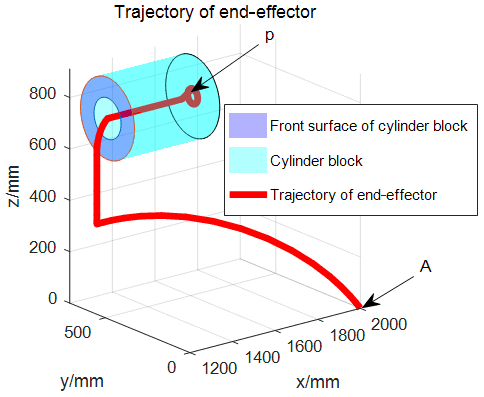
To verify the mapping relationship between the flexible cable drive space and the joint rotation space for the hyper-redundant manipulator, the initial length change for each flexible cable was set to 0 mm, the initial angle of each joint was set to 0^∘, and the rotation angle range for each joint was set to [−45^∘, 45^∘]. The total length of the hyper-redundant manipulator was 2000 mm. The initial spatial coordinate position of end-effector A was (2000, 0, 0). A thin-walled cylindrical oil tank was assumed to exist in the working space. The upper and lower walls of the oil tank were circles with radii of 160 mm. The center of the circle on the upper wall was at (1250, 550, 751), the center of the circle on the lower wall was at (1650, 550, 751), and the height of the oil tank was 400 mm. There was a circular opening with a radius of 80 mm on the upper wall of the tank, and there was a circular opening, P, with a radius of 30 mm on the tank's lower wall. The simulation process required the hyper-redundant manipulator to pass through the oil tank's upper and lower openings and through its inner wall to achieve the track operation of the circular opening, P. During this process, the hyper-redundant manipulator must not touch the underside openings or the tank walls. For different trajectory planning, the changes in the hyper-redundant manipulator's joint angles would be different, resulting in different trends for the cable lengths. Therefore, different cable length change trends could be obtained through complex trajectories, which could improve the accuracy of the formula verification. Through the comprehensive application of a quintic polynomial (Hu et al., 2018; Chettibi et al., 2019), a spatial linear interpolation algorithm, a spatial circular interpolation algorithm, and the trajectory planning for the hyper-redundant manipulator, the trajectory of the hyper-redundant manipulator's end-effector was obtained for the whole working process, as shown in Fig. 5. The trajectory curve was continuous and stable and effectively avoided touching the openings and inner surfaces of the upper and lower walls of the cylindrical tank. It smoothly entered the inside of the cylindrical tank and reached the lower wall, thus achieving the planned trajectory of the circle P.

Figure 5 The trajectory of the end-effector.

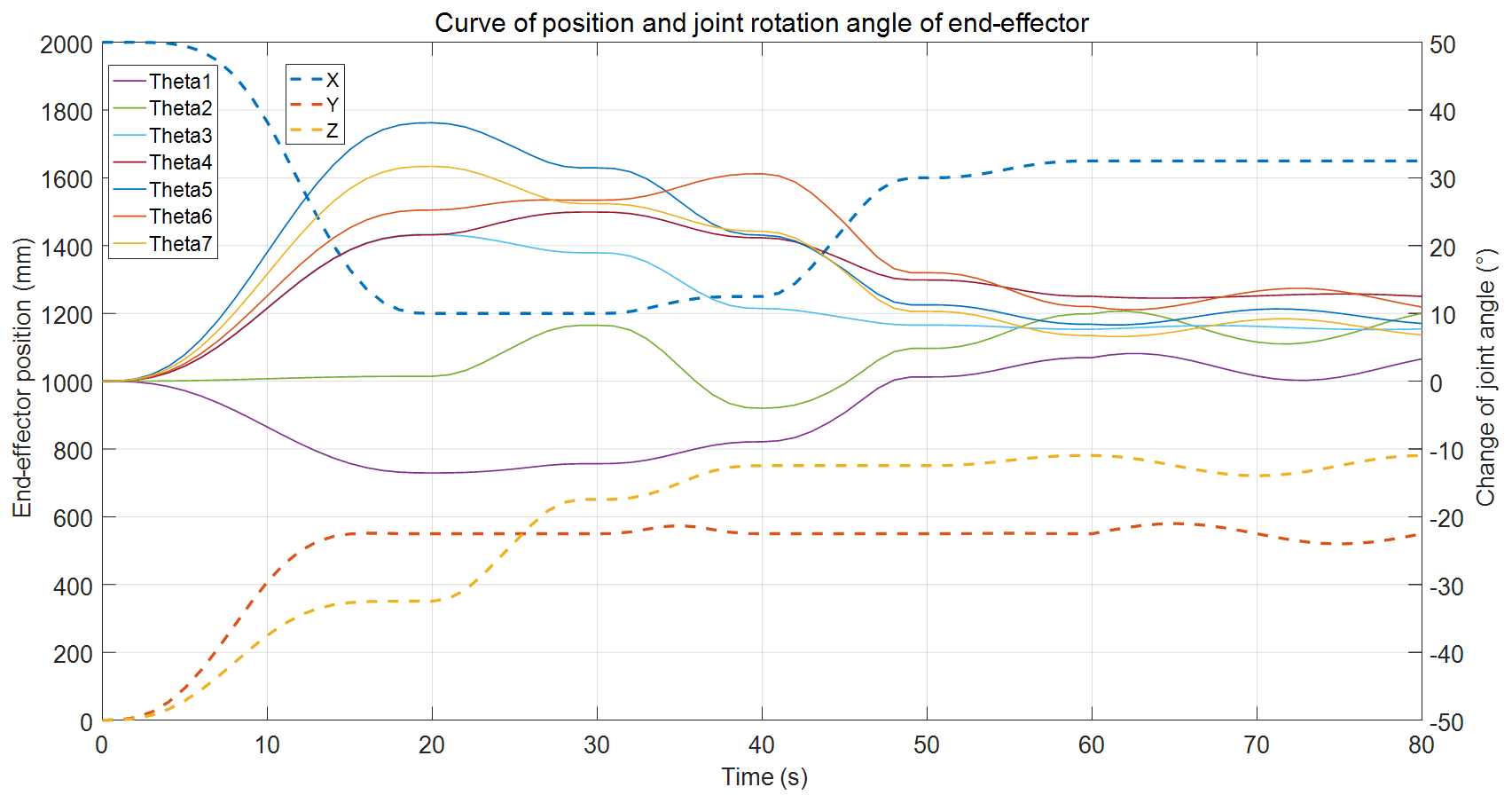
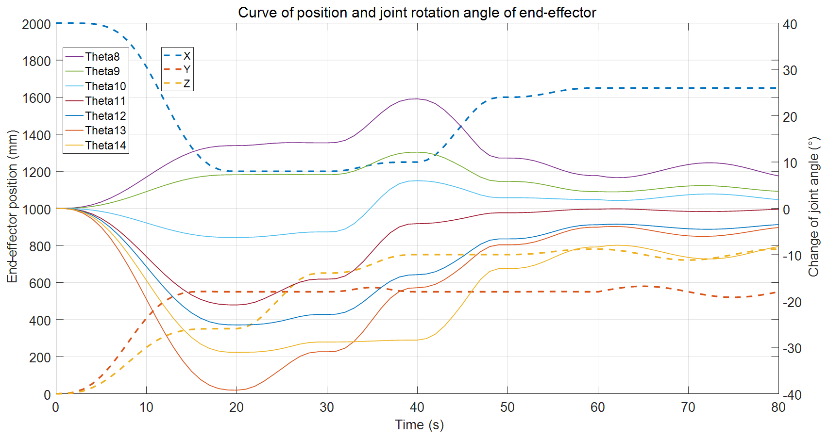
Figures 6–8 show the end-effector's coordinate and joint rotation angle change curves. During the whole movement process, the maximum clockwise rotation angle was 38.121^∘, occurring for Theta5 at 20 s, and the maximum counterclockwise rotation angle was −39.236^∘, occurring for Theta13 at 20 s. The overall range of angle changes for the hyper-redundant manipulator was [−39.2360^∘, 38.121^∘]. The joint rotation angles' variation range was smaller than its spatial range, and it met the robot joint motion requirements. The angle changes for each joint produced relatively smooth curves, and the sudden changes in the joints' angular velocity and angular acceleration were avoided in the joint space, which ensured good motion performance.

Figure 6 End-effector coordinates and joint angle curves (1).

Figure 7 End-effector coordinates and joint angle curves (2).

Figure 8 End-effector coordinates and joint angle curves (3).

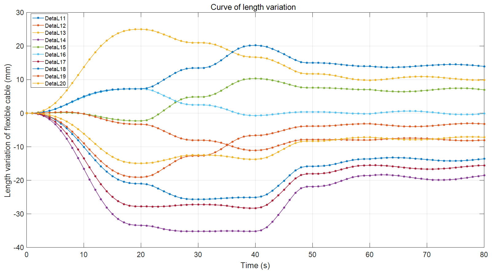
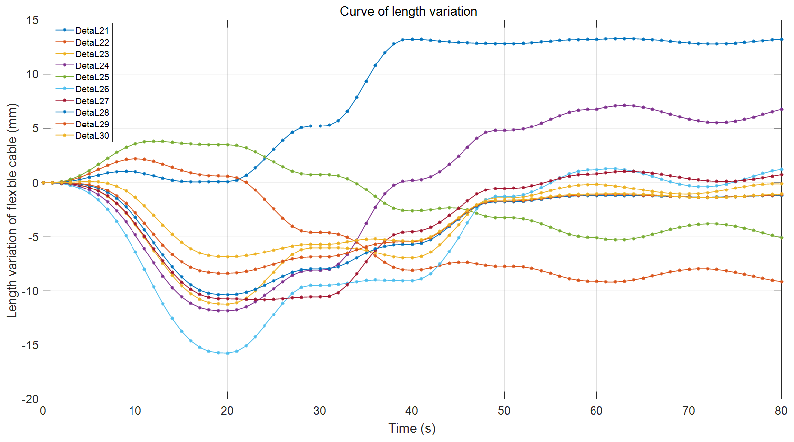
Figures 9–11 show the curves representing the changes in the lengths of the cables. The maximum shrinkage length, −35.1981 mm, occurred for DetaL14 at 30 s, and the maximum stretching length, 29.6284 mm, occurred for DetaL10 at 23 s. The variation range was [−35.1981 mm, 29.6284 mm], which provided a reference for the driving motor's sliding stroke. The changes in each cable's length produced smooth curves because of the avoidance of sudden changes in motor speed and acceleration. A comparison of Figs. 6–8 and 9–11 showed that a larger range of angle changes corresponded to a larger range of joint length changes, which aligned with the motion law and the mapping relationship driven by the flexible cable.

Figure 9 Flexible cable length variation curves (1).

Figure 10 Flexible cable length variation curves (2).

Figure 11 Flexible cable length variation curves (3).

The cable length variations were substituted into Eq. (13) to obtain the rotation angles for each joint. These joint rotation angles were substituted into the robot kinematics equation established by the D–H parameter method (Zhang et al., 2016) for the forward solution analysis to obtain the hyper-redundant manipulator's trajectory curve. Figure 12a–d show the positions of the hyper-redundant manipulator during the time periods of 0–20, 20–40, 40–60, and 60–80 s, respectively, from the initial point to the end point, where the sampling time interval between adjacent poses was 1 s.

Figure 12 Simulation results of trajectory planning for the hyper-redundant manipulator.

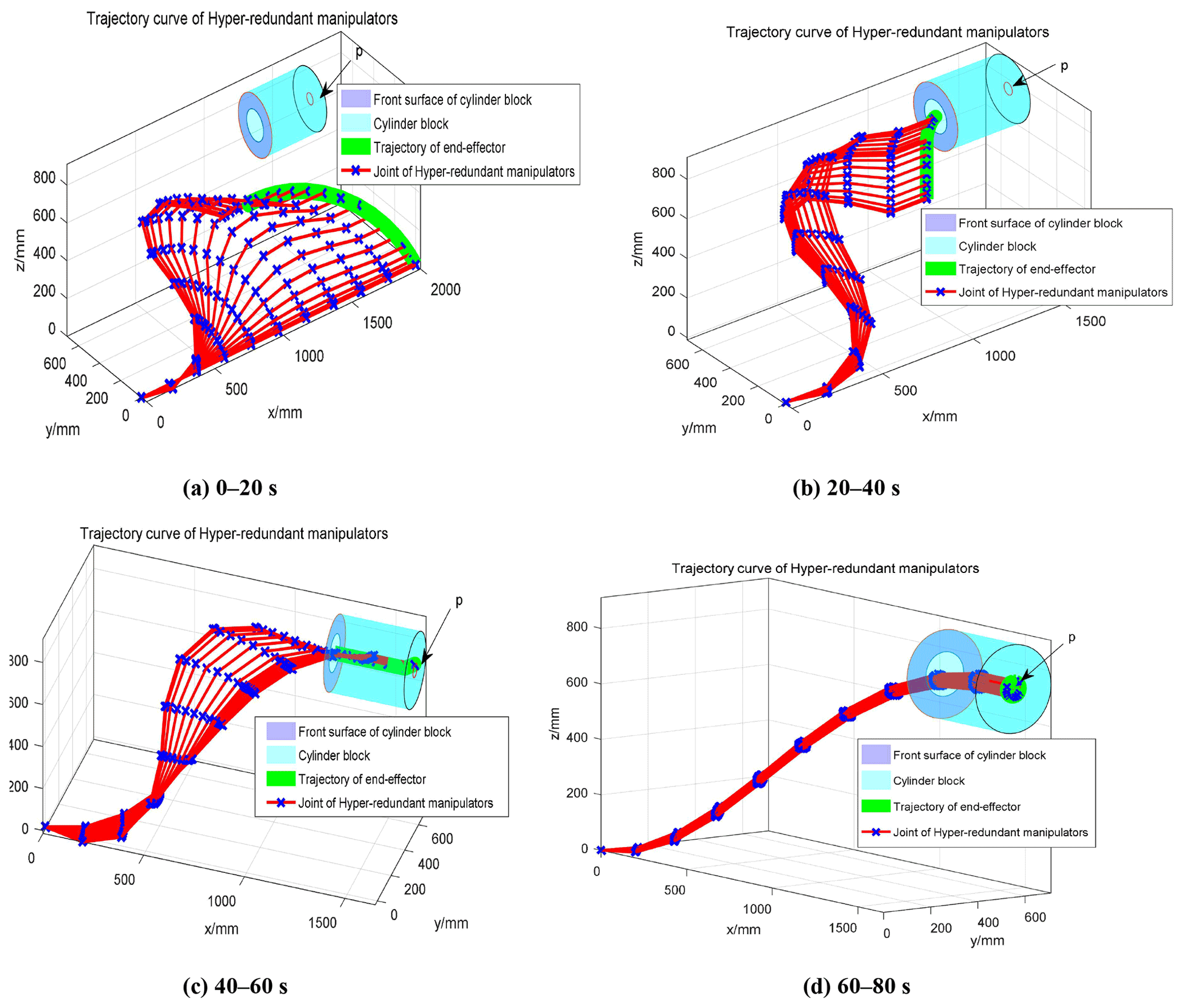
A comparison of Fig. 12 with Fig. 5 indicated that the trajectory curves obtained for the end-effector were essentially consistent, thus proving the appropriateness of the coupling analysis for each of the hyper-redundant manipulator's joints. Therefore, Eq. (13) could be used to effectively convert each joint angle and perform cable length transformations for the hyper-redundant manipulator, and thus the mapping relationship between the cable drive space and the joint rotation space could be obtained. These results can provide a theoretical basis for the design of the drive spaces and the joint rotation spaces of hyper-redundant manipulators.

6 Conclusions

1. To solve the kinematics mapping problem for the joint space and the drive space of a hyper-redundant manipulator based on flexible cable actuation, which is the key for hyper-redundant manipulators to move strictly according to trajectory planning and avoid obstacles, a decoupling method for kinematics analyses of the flexible cable actuation space and the joint rotation space was proposed. It effectively solved for the influence of coupling between the joints of the flexible cables on the drive control. Thus, the mapping relationship between the variation law of the cables' lengths and the variation law of the joints' rotation angles was obtained.

2. The research results show that the actual joint angles of the hyper-redundant manipulator driven by flexible cables met the set angle range and that the change rules for the flexible cables and angles were smooth curves. This indicated an avoidance of sudden changes in angular velocity and angular acceleration for all joint angles and the prevention of motor jitter and even impact caused by discontinuous acceleration. A larger variation range for the cable length changes corresponded to a larger variation range for the rotation angle changes, which accorded with the motion law and mapping relationship of the cable drive and provided a theoretical reference for the establishment and sliding stroke of the drive motor.

3. Based on trajectory planning of a higher-order polynomial, spatial linear and spatial arc interpolation algorithms were used to solve the trajectory of the hyper-redundant manipulator's end-effector. The change law for each of the robot's joint angles was obtained based on the pseudo-inverse Jacobian matrix, and the change law for each drive cable was solved based on the decoupling analysis method. The change law was substituted into the forward kinematics solution to solve for the spatial trajectory of the robot, and the appropriateness of the proposed decoupling analysis method was verified. Additionally, a solution strategy for the flexible cable-driven hyper-redundant manipulator to achieve a predetermined trajectory was presented. The simulation results verified the acceptability of the method and strategy. According to the robot's specific trajectory planning scheme, this method led to precise control of the driving cables' length changes and the joint angles' changes and finally caused the end-effector to arrive at the operation point with high precision. This study provides a technical and theoretical reference for precise control, trajectory planning, and obstacle avoidance for a cable-driven hyper-redundant manipulator.