Horizontal axis wind turbine modelling and data analysis by multilinear regression

The modelling of each horizontal axis wind turbine (HAWT) differs due to variation in operating conditions, dynamic parameters, and components. Thus, the choice of profiles also varies for specific applications. So for the better choice of profiles, the wind turbine performance is analysed for different parameters and working conditions. The efficiency of HAWTs mainly depends on the blade, which in turn is related to the profile of the blade, blade orientation, and tip size. Hence, the main aim of the present work is to evaluate the performance of HAWTs for three different blade tip sizes and six different blade twist angles for three major NACA (National Advisory Committee for Aeronautics) airfoils. A statistical analysis is also carried out to find the influence of different performance parameters such as drag, lift, vorticity, and normal force. The static design parameters are considered based on the available literature. A three-bladed offshore HAWT is adopted as the research object in the study. Data visualization using star glyphs and sunray plots is performed, along with multilinear regression analysis. From the multilinear regression analysis and reliable empirical correlations, it is known that drag coefficient and lift coefficient parameters have less significance in contrast to the other parameters which have more significance in the regression model. The different results obtained in terms of parametric coefficients provide an effective way to generate appropriate airfoil profiles for given HAWTs. Thus, the study helps to achieve better turbine performance, and it serves as a benchmark for future studies on HAWTs.

1 Introduction

Wind energy is a renewable resource that can be used to generate electricity. As fossil fuels are getting depleted, this wind energy could be utilized on a large scale for producing electricity. Wind energy is also suitable for reducing greenhouse gas effects, and it fulfils future energy needs. The latest research in this field mainly focuses on the potential of turbine blade technology in providing effective performance. Wind turbines are classified into horizontal axis wind turbines, vertical axis wind turbines, and small axis wind turbines. Horizontal axis wind turbines with horizontal rotating shafts are used from small windmills to large-scale commercial wind turbines. Vertical axis wind turbines with vertical shafts are utilized for various purposes and are based on the Savonius rotor, the Darrieus rotor, and the H rotor. Small axis wind turbines are used for small-scale utilities like in households and for industrial research.

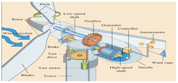
Horizontal axis wind turbines (HAWTs) produce electricity by the rotation of wind turbine blades whereby the axis of rotation is parallel to the wind stream. Thus, a high amount of electricity is generated with lower wind speeds. HAWTs are equipped with a good starting performance at high rotating speeds (Hau, 2006). The control of the rotor is related to wind speed, and at higher wind speeds the turbine blades are controlled with the assistance of pitch and yaw of the blade in the self-starting module. Consequently, for every 10 m of wind speed rise, the power output increases by about 34 % with the assistance of the control mechanism (Leble and Barakos, 2017). In the case of vertical axis wind turbines (VAWTs), the rotor is uncontrollable during high winds and requires huge space with a low tip speed ratio. As VAWTs are shorter and are placed at lower heights from the ground, thin wind flow on the ground creates turbulent flow and high vibration (Dominy et al., 2007). Hence, HAWTs are prioritized and utilized at a large scale.

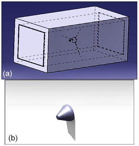
HAWTs are classified based on the number of blades, the shape of the tower, and the offshore and onshore location. Freere et al. (2010) experimented with the low-cost three-bladed wind turbine for a case study with a rotor diameter of 2.1 m. The wind turbine was tested at a wind speed of 13 m s⁻¹. The results provided better operation of the wind turbine. For a tip speed ratio of 5, the maximum power coefficient attained was 0.2 (Freere et al., 2010). Singh et al. (2011) utilized the conical tower for the design and analysis of the rotor, as a conical-tubed tower can withstand heavy wind with an increase in strength. The designed rotor was estimated to generate power of about 750 KW for a blade length of 21 m under upwind conditions. The deflection and stresses in the blade were estimated. The estimated deflection occurring at the blade root was about 0.69433, and the maximum stress obtained was 81.13 MPa (Singh et al., 2011). Feyzollahzadeh et al. (2016) studied the offshore wind turbines and then applied a finite element method (FEM) and a transfer matrix method (TMM) to estimate the dynamic loading and axial induction factor. TMM displayed a better model for the estimation of the dynamic response of a 1 MW offshore wind turbine, under thrust and unbalance forces for a tower height of 91.44 m, a tower thickness of 9.525 m, and for a rotational speed of 20 rpm (Feyzollahzadeh et al., 2016). The number of blades and tower height are required to evaluate the tip speed ratio and performance parameters, like the pressure, force, velocity, and vorticity of HAWTs. Hence a three-bladed conical offshore wind turbine is chosen as the research object in our study. Figure 1 shows the three-dimensional model of an offshore three-bladed conical tower wind turbine (Ahmad, 2019).

Figure 1 3-D view of the commercial horizontal axis wind turbine.

A high lift-to-drag ratio is required for efficient turbine performance (Burton et al., 2001). Few researchers have contributed their efforts to optimizing the blade geometry using mathematical correlations and simulation of the blade using computational fluid dynamics and Fluent software. Mathematical correlations include performance and premier design of comparative sizes of the HAWT blade geometry with data analysis using a multilinear regression method. Multiple linear regression analysis is a predictive analysis in which the data are analysed by using different independent variables and one dependent variable. This regression model is the extension of ordinary least squares regression. The key contribution of our work as follows: to design the HAWT blade geometry based on mathematical correlations. Then the HAWT blade design data are analysed using a multilinear regression method. The predictive analysis of regression utilizes independent and dependent variables. This regression model is evaluated with dependent variables, independent variables, intercept values, slope coefficients, and residuals. Data visualization using star glyphs and sunray plots is performed, along with multilinear regression analysis.

2 Literature survey

Several approaches are adopted to evaluate the performance of horizontal axis wind turbines and analyse data through different types of regression analysis. Li et al. (2020) found that large horizontal axis wind turbines have high efficiency and also reduce the cost of energy by implementing a suitable wind turbine blade design. In order to achieve high aerodynamic efficiency and reduction in noise, a modified mathematical framework was proposed by including overall design optimization. The results displayed an increased lift-to-drag ratio. Sayed et al. (2012) estimated the various wind turbine blade profiles in such a way that it improved the power of the wind turbine by finite volume numerical calculations. The wind turbine blade profile was modified with respect to chord length, span, pressure side, and suction side of the airfoil in order to attain the maximum power. The range of the tip speed ratio was taken from 5 to 7 and the optimum angle of attack as −4 and 3^∘. For these angles of attack, the results showed that the most efficient blade profiles were S825, S826, S830, and S831 as per the working conditions at low and high wind speeds. Devinant et al. (2002) studied the effect of turbulence on the airfoil NACA 0012 (National Advisory Committee for Aeronautics) through qualitative and quantitative analysis. The airflow on the surface of the airfoil got separated due to high turbulence created on the airfoil. This resulted in reduced lift force on the wing of airfoil NACA 0012. Lift coefficient and drag coefficient variation in the airfoils were analysed particularly with the angle of attack. The 0 to 90^∘ range was considered, and the results displayed an increase in the lift coefficient for 0 to 15^∘, whereas the drag coefficient increased from 15^∘. Sicot et al. (2008) stated that the turbulence and wind speed have a significant effect on the lift and drag coefficients that drive the wind turbine aerodynamics. Tests were conducted under a wind tunnel with a varying turbulence of 4.5 % to 12 % for high wind speeds. The steady separation point provided necessary improvement in the lift coefficient of the wind turbine blade. Himmelskamp (1947) investigated the pressure distribution and coefficient of pressure that were caused due to the stall delay within the rotation and increase in lift coefficient. The lift coefficient was determined from radial flow and the pressure distribution along the profile of the inner blade. However the effects of Coriolis force were ignored around the blade profile. Thus, the lift coefficient values increased with positive angle of attack (Riziotis and Voutsinas, 1997). Premalatha and Rajakumar (2016) studied the aerodynamic characteristics of the wind turbine blades using ANSYS Fluent software. The experiments were conducted with and without a winglet in the rotor blades. The results showed that by altering the height of the winglet, the power coefficient increased, and the radius curvature of the blade decreased. Ockfen and Matveev (2009) studied the aerodynamic characteristics of the NACA 4412 airfoil with flaps to estimate the lift coefficient with respect to the ground effect. The results showed that for the wind turbines with flaps, there was an overall increase in lift coefficient and up to a 5 % increase in chord length. Also, the highest lift-to-drag ratio was obtained for a flap deflection of 2.5 %.

A completely optimized profile requires consideration of the blade tip size and air foils. Castellani et al. (2006) studied different wind flows in farm wind turbines in hilly areas, located in regions of the Netherlands, with different blade tip sizes. The results showed a 5 % rise in the overall power coefficient of the wind turbine with respect to rise in the lift-to-drag ratio. Abrar et al. (2014) proposed an optimization technique and blade tip shape design modification for the horizontal axis micro wind turbine to attain self-rotation without external aid. This was achieved at a high tip speed ratio, as the high tip speed ratio and blade pitch angle increased the power coefficient and overall performance of the wind turbine. In phase 6 of the National Renewable Energy Laboratory (NREL), Ferrer and Munduate (2017) evaluated the blade pitch axis and a swept-back tip mathematically using Fluent 6.2 and proved that the pitch axis at the tip worked relatively well. The radial flow was altered by the blade tip shape and was justified by the three-dimensional effects of the load acting on the blade. This resulted in a rise in efficiency of the wind turbine by shift of the blade momentum within the inboard sections. Tahani et al. (2017) enumerated wind turbine geometrical parameters like length of the chord, angle of twist, and 40 other different parameters which optimize the power of the wind turbine. The power can be increased by about 13.7 % by analysing 40 geometrical parameters of the horizontal axis wind turbine. Performance evaluation of NACA 0012 was conducted in CFD software with turbulence models. A standard K-□ SST turbulence model was used for the computational evaluation. The results displayed that, for a 10 m s⁻¹ rise in wind speed, there was about a 10 % increase in power of the wind turbine (Kumar et al., 2013). Ashrafi et al. (2015) increased the power coefficient parameter for a horizontal axis wind turbine with 200 KW power generation. This was achieved with the optimization of pitch angle with respect to wind speed for different twist angles. Sharifi and Nobari (2013) proposed an algorithm to evaluate the blade section pitch angle along the wind turbine blade to extract the maximum power from the wind turbine at the installation site. Code was written based on blade element momentum (BEM) theory, and it estimated the precise power generated by controlling the aerodynamics of the HAWT. The power generated in the test wind turbine was about 14.42 KW, which was about a 22.01 % increase from the existing wind turbine. Uyanik and Guler (2013) studied the multilinear regression analysis based on their assumptions related to study parameters at Sakarya University, Turkey. Based on the results, they improved the education system in the university by taking five independent variables and dependent variables based on ANOVA statistics.

The intention of the study is to evaluate the performance of the wind turbine blade profiles in order to find a suitable NACA blade profile for Indian wind conditions. From the literature survey, two major factors considered are wind turbine blade design and wind flow conditions. However, the second factor is uncontrollable, and the first factor should be well defined to maximize the power of the wind turbine. In this regard, the research carried out by Tahani et al. (2017) focused their discussion on the six chord distribution functions and six twist parameters for 12 airfoils and evaluated the performance parameter of turbulence intensity. Hence, CFD is utilized for the simulation of the wind turbine blade. It determines the performance parameters of turbulence intensity and power of the turbine. However, the influence of geometry is restricted only to determine the single performance parameter of turbulence intensity. In order to bridge the gap, performance analysis of the blade geometry with six twist angles, three tip sizes, and three NACA airfoils is considered for the case of large HAWTs in this paper.

The selection of airfoil is a key factor in wind turbine design. Oukassou et al. (2019) conducted a study to determine the best among the two airfoils NACA 0012 and NACA 2412, with the help of ANSYS Fluent 16.2. The main objective of the study was to determine the twist and chord distributions for the design of wind turbines and to obtain a maximum lift-to-drag ratio. Lift and drag coefficient, lift-to-drag ratio, and power output were calculated and compared. It is observed that NACA 2412 exhibited a maximum power output as compared to NACA 0012. In order to develop sophisticated wind turbines for the Indian market, comparative analysis for NACA 0012, NACA 4412, and NACA 4415 is considered in the current research work to obtain better performance results.

The other researcher, El Chazly (1993) analysed the aerodynamic forces and torque created on the rotor blade, with different twist angles of the blades ranging from 7 to 40^∘. The results displayed that the twisting of blade improved the stiffness and the strength of the blade. Gudmundsson (2014) explained the anatomy of the four-digit airfoils and determined the significance of each digit in the NACA four-digit series airfoil. The turbulent boundary layer was also evaluated along with the effects of wind flow separation. Accordingly, in this paper, six different twist angles are taken and the performance parameters are compared along with three airfoils and three blade tip sizes. Sedighi et al. (2020) presented a numerical investigation of the V47-660KW HAWT. The wind turbine suction sides were altered with spherical dimples. The models of shear stress and turbulent transport Reynolds-averaged Navier–Stokes solver were utilized to solve the momentum equations. The wind speed and blade pitch angle effects were examined to achieve the best dimpled blades. The generated torque was enhanced by 16.08 %. Seyednia et al. (2019) investigated the dynamic performance of the HAWT-based dynamic stall (DS). Reynolds-averaged Navier–Stokes equations were utilized to simulate the deformable trailing-edge flap (DTEF). DS vortex, size, and strength are influenced through DTEF phase defection. Most effectively, a change in the airfoil camper-line in flap oscillation can significantly distress the pressure distribution nearby the aircraft, thus achieving a significant load reduction and average lift development. In the parameter study, the DTEF is compared with the discrete flap based on the defection amplitude and size. Fatigue load control in relation to the airfoil with a similar amplitude and frequency of up to 30 % of the total coin oscillation was outside the phase of the slowly curved DTEF.

Based on the request of the National Institute of Wind Energy (NIWE), India, for an EOI (expression of interest) for the installation of the first 1000 MW commercial offshore wind farm at Jafarabad in Gujarat, the wind speed of 36 m s⁻¹ is selected for a hub height of 80 m, by comparing the mast wind data available from the NIWE. However, Neill and Hashemi (2018) discussed the minimum and maximum wind speeds in the range of 0 to 36 m s⁻¹. They also discussed ocean renewable energy for which wind speeds are recorded for every single hour, and these observations were taken as bins. Hence, in the current work, maximum wind speed is taken and compared for the three NACA airfoils, and the best airfoil is determined by using statistical analysis and multilinear regression analysis.

In the current research work, the numerical simulation of three airfoils (NACA 0012, NACA 4412, and NACA 4415) was performed to evaluate the performance parameters drag, lift, normal force, dynamic pressure, relative pressure, turbulence intensity, torque, axial velocity, and vorticity. This was achieved by

1. setting the number of blades and rotor diameter as input parameters and

2. finding the optimal profile for the blade twist angles of 0, 3, 6, 9, 12, and 15^∘, with blade tip sizes of 0.1, 0.15, and 0.2 m.

Nowadays, there is a paradigm shift towards the modification of the blade twist angle and blade tip size to obtain the maximum performance of the HAWT. Hence, the following is important.

• The rotor and blade assembly 3-D flow simulation is performed by wind tunnel test, and the two-dimensional airfoil simulation is done with ANSYS Fluent 19.1.

• The airfoils NACA 0012, NACA 4412, and NACA 4415 are simulated for different blade tip shapes and blade twist angles, and results are recorded carefully.

• The data visualization is performed including star glyphs and sunray plots, and multilinear regression analysis is performed.

3 Numerical model

3.1 Configuration

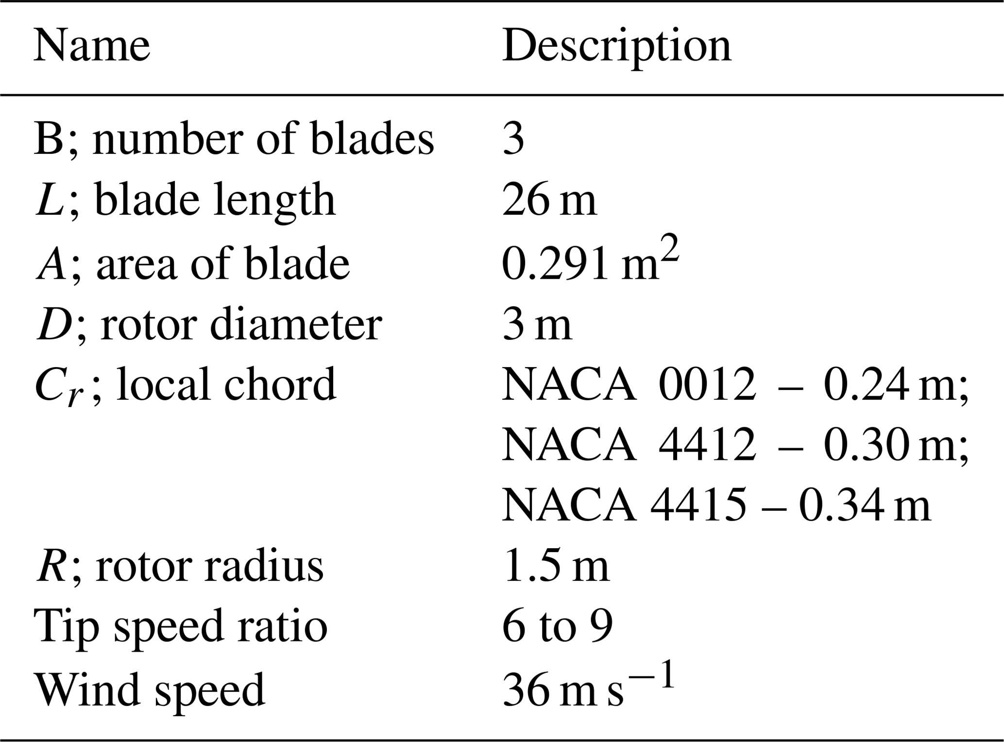
In this research, two-dimensional airfoil simulation is carried out with six different blade twist angles. The blade twist angles taken are 0, 3, 6, 9, 12, and 15^∘. The output of these blade twist angles is recorded, and the optimal airfoil is selected out of NACA 0012, NACA 4412, and NACA 4415 airfoils using data visualization techniques. Three-dimensional rotor and blade assembly simulation is performed in a wind tunnel, in which different blade twist angles and blade tip shapes are taken as static parameters. The blade tip shapes of 0.10, 0.15, and 0.20 m are considered along with the blade twist angles. These different blade tip shapes and blade twist angles help in finding out the optimal blade for HAWTs. The tip speed ratio is also considered as a static parameter in designing the wind turbine blades. The design of a horizontal axis wind turbine is based on the amount of wind energy the turbine blade can extract from the wind. A detailed view of available HAWT configurations and the work done on each configuration have been discussed in the following sections. Table 1 provides the data of the HAWT parameter specifications that are used in the current research.

Table 1 HAWT parameter specification.

3.2 Numerical simulations

Boundary conditions and meshing of the virtual model ease the simulation process, and a valid optimal airfoil could be achieved. In this research, BEM theory is utilized in which the blade is divided into equal parts to estimate the forces involved in converting the kinetic energy of the wind to electric energy. By assuming airfoil strips with minuscule thickness which are aerodynamically independent with zero interference between airfoils, as per BEM theory (Sharifi and Nobari, 2013), axial force and thrust force can be obtained using Eqs. (1) and (2).

$$\begin{array}{}\text{(1)}& {\displaystyle }\mathrm{d}F=\mathrm{1}/\mathrm{2}{\mathit{\rho }}_{\mathrm{a}}BC{W}^{\mathrm{2}}\mathrm{d}r[C_{\mathrm{L}}\cos \mathit{\varnothing }+C_{\mathrm{D}}\sin \mathit{\varnothing }]\text{(2)}& {\displaystyle }\mathrm{d}F=\mathrm{1}/\mathrm{2}{\mathit{\rho }}_{\mathrm{a}}BC{W}^{\mathrm{2}}\mathrm{d}r[C_{\mathrm{L}}\sin \mathit{\varnothing }-C_{\mathrm{D}}\cos \mathit{\varnothing }],\end{array}$$

where B is the number of blades, I the inflow angle, W the resultant velocity, C the airfoil chord, and C_L and C_D the lift and drag coefficients respectively.

In order to achieve reliable results through the simulation process, it is important to apply the right meshing method and boundary conditions. Meshing is the process of dividing the complex component into small equal parts so that the problem solving method can be easily applied in each small part. This meshing process is followed in order to acquire optimal results by evaluating the numerical equations based on boundary conditions. However, the boundary conditions are the input parameters provided to the inlet, outlet, and wall. These boundary conditions should be precise and validated. The numerical simulations in this paper are conducted using ANSYS Fluent 19.1 and SOLIDWORKS Flow Simulation software. However, the multilinear regression analysis is done in RStudio.

3.3 Wing geometry and fluid domain

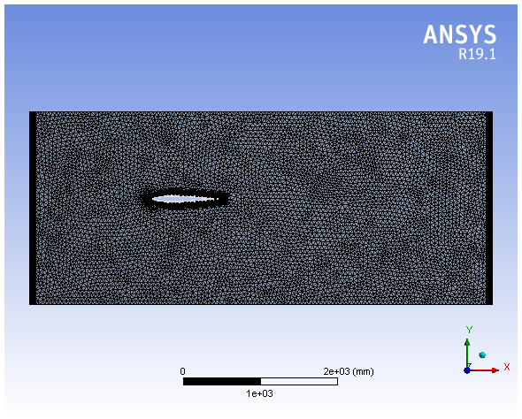
Wing geometry is based on the NACA coordinates for each airfoil and consists of the leading edge, trailing edge, span, chord length, and camber line. The upper wing of airfoil NACA 0012 is symmetric with the lower wing, whereas for airfoils NACA 4412 and NACA 4415, the upper wing of the airfoil is not symmetric with the lower wing of airfoil. For a symmetric airfoil (NACA 0012), the effects of performance parameters are similar on the pressure side as well as the suction side. In contrast, for non-symmetric airfoil (NACA 4412 and NACA 4415), the effects of performance parameters are dissimilar on the pressure side and suction side. Each airfoil is enclosed in a rectangular section. This enclosure helps in creating the necessary fluid domain. The mesh is generated on the wing and rotor based on the C-type grid topology. This assists in developing a better flow around the wing.

3.4 Procedure for ANSYS

Two-dimensional analysis is performed with ANSYS Fluent to obtain a precise result. The design and analysis methodology is displayed in the figures below. In the current analysis, viscous flow is used with a hybrid initialization solution technique with second-order upwind momentum based on the least-squares-cell-based gradient (Sharifi and Nobari, 2013). Mesh is generated in ANSYS Fluent 19.1 as shown in Figs. 2 and 3. The boundary conditions applied within ANSYS Fluent 19.1 are inlet velocity and environment pressure. At a wind speed of 36 m s⁻¹ for the inlet velocity, the parameters pressure coefficient, lift coefficient, drag coefficient, lift-to-drag ratio, vorticity, turbulence intensity, static pressure, dynamic pressure, and torque, etc., are recorded as output parameters.

Figure 2 2-D airfoil generated with point NACA 0012 at a 0^∘ blade twist angle.

Figure 3 2D meshed airfoil for Fluent analysis for NACA 0012 at a 0^∘ blade twist angle.

Procedure for CAD modelling

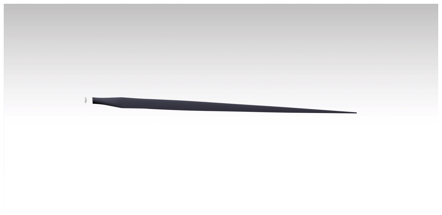
Three airfoils, NACA 0012, NACA 4412, and NACA 4415, are designed, and simulation is carried out with different blade tip sizes of 0.1, 0.15, and 0.2 m along with twist angles of 0, 3, 6, 9, 12, and 15^∘. Simulation is done in a wind tunnel test. One end of the wind tunnel is considered with an inlet wind speed of 36 m s⁻¹ and the other end with environmental pressure conditions. The environmental conditions taken are 101 325 Pa pressure and a temperature of 293.20 K. These environmental conditions are based on upwind conditions of the offshore wind turbine. For the airfoils NACA 4412, NACA 4415, and NACA 0012 three-dimensional designs of rotor and blade are performed in the CAD package as shown in Fig. 4. Figure 5 shows the three-dimensional model of the blade, and Fig. 5a shows the three-dimensional rotor model. The design is validated with appropriate measures.

Figure 4 3-D model of the blade.

Figure 5 (a) 3-D model of the rotor. (b) Assembled blade and rotor in the wind tunnel.

3.5 Regression analysis equations

There are many different regression analyses to analyse and interpret the data obtained. Among them, the multilinear regression model is the most prominent for multiple independent variables (inputs) and single dependent variable (output). The dependent variable is always analysed based on n, the number of independent variables. Here in our research, the blade angle, the blade tip size, and the NACA profile are said to be independent variables that influence the dependent variables like drag, lift, and normal force.

The general multilinear regression model is given below as Eq. (3):

$$\begin{array}{}\text{(3)}& Y_i={\mathit{\beta }}_{\mathrm{0}}+{\mathit{\beta }}_{\mathrm{1}}{X}_{\mathrm{1},i}+{\mathit{\beta }}_{\mathrm{2}}{X}_{\mathrm{2},i}+{\mathit{\beta }}_{\mathrm{3}}{X}_{\mathrm{3},i}\mathrm{\dots }+{\mathit{\beta }}_p{X}_{p,i}\mathrm{\neg }+{\mathit{ϵ}}_i,\end{array}$$

where Y is the dependent variable, X_i is the independent variable, and ϵ is the error which is formed due to the dependent variable. β is the intercept or the slope coefficient. However, the matrix form is utilized to estimate the mean value of the dependent variable. Estimation of the error variance is done in two ways, that is

• in the form of vector and matrix notations and

• by implementing the linear model in the matrix form given by Eq. (4):

$$\begin{array}{}\text{(4)}& Y=X\mathit{\beta }+{\mathit{ϵ}}_{\mathrm{1}}E\left(\mathit{ϵ}\right)=\mathrm{0}.\end{array}$$

From Eq. (4), β can be interpreted. There is also another method of estimating the β value by taking the estimation of the β as shown in Eq. (5):

$$\begin{array}{}\text{(5)}& E\left(\widehat{\mathit{\beta }}\right)=\mathit{\beta }.\end{array}$$

Here $\widehat{\mathit{\beta }}$ is the estimation of β, which is also termed “BLUE” (best linear unbiased estimate).

3.5.1 Multiple correlation coefficient

The multiple correlation coefficient is predicted for the dependent variables Y and is given as Eq. (6).

$$\begin{array}{}\text{(6)}& \mathrm{Cor}(Y,\widehat{Y})={\displaystyle \frac{\mathrm{\Sigma }(Y_i-\stackrel{\mathrm{‾}}{Y})(\widehat{Y_i}-\widehat{Y})}{\sqrt{\mathrm{\Sigma }(Y_i-\stackrel{\mathrm{‾}}{Y}{)}^{\mathrm{2}}\mathit{\sigma }(\widehat{Y_i}-\widehat{Y}{)}^{\mathrm{2}}}}}\end{array}$$

The numerator gives the sum of all dependent variables, and the denominator gives the normalization.

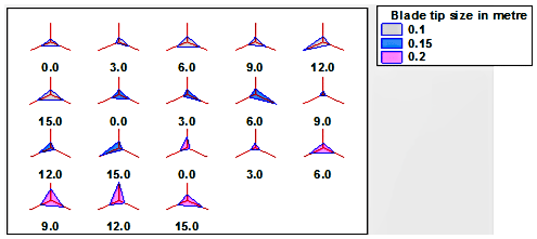
Figure 6 Sunray plot for turbulence intensity with different blade tip sizes of 0.1, 0.15, and 0.2 m and blade twist angles of 0, 3, 6, 9, 12, and 15^∘ for three airfoils.

Figure 7 Turbulence intensity for three airfoils NACA 0012, NACA 4412, and NACA 4415.

3.5.2 Coefficient of determination R²

The coefficient of determination R² is given in Eq. (7).

$$\begin{array}{}\text{(7)}& R^{\mathrm{2}}=\mathrm{1}-{\displaystyle \frac{\mathrm{SSE}}{\mathrm{SST}}}=\mathrm{1}-{\displaystyle \frac{\mathrm{\Sigma }(Y_i-\widehat{Y_i}{)}^{\mathrm{2}}}{\mathrm{\Sigma }(Y_i-{\stackrel{\mathrm{‾}}{Y}}_i{)}^{\mathrm{2}}}}\end{array}$$

Here, the SSE denotes the sum of square of errors. SST denotes the sum of the square total.

3.5.3 Adjusted R²

Adjusted R² is given as $R_{\mathrm{a}}^{\mathrm{2}}$ and is shown in Eq. (6). The model is said to be fit. In the case that the numerator is close to zero, then R² will be 1.

$$\begin{array}{}\text{(8)}& R_{\mathrm{a}}^{\mathrm{2}}=\mathrm{1}-(\mathrm{SSE}/(n-p-\mathrm{1}\left)\right)/(\mathrm{SST}/(n-\mathrm{1}\left)\right)\end{array}$$

Here, $(n-p-\mathrm{1})$ is the given degrees of freedom. n−1 is the offset for the degrees of freedom.

Table 2 Data variables for turbulence intensity.

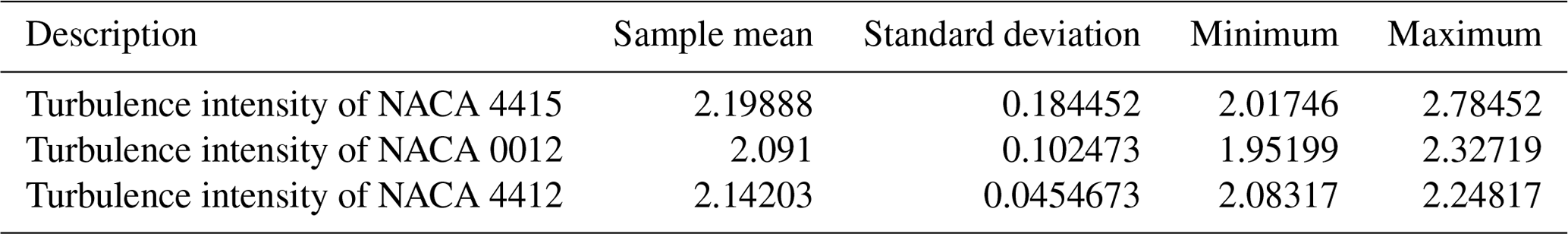
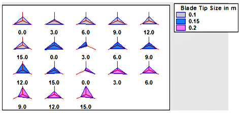
Figure 8 Sunray plots with values of static pressure blade tip sizes of 0.1, 0.15, and 0.2 m and blade twist angles of 0, 3, 6, 9, 12, and 15^∘.

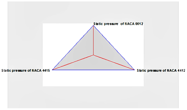
Figure 9 Star glyph showing static pressure for three airfoils, NACA 0012, NACA 4412, and NACA 4415.

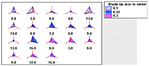
Figure 10 Vorticity values are displayed for NACA airfoils for three different blade tip sizes and six different blade twist angles.

Figure 11 Star plot showing vorticities for NACA airfoils.

3.5.4 R program data

The set of steps written in the R program is given below.

•  

  head(file name)

•  

  pairs (file name[1:2:3:4])

•  

  summary(file name)

•  

  #Multiple Linear Regression

•  

  results ← lm(file name independent variable1+ independent variable2+ independent variable3, file name)

•  

  results

•  

  summary(results)

•  

  reduced ← lm(file name independent variable1+ independent variable2+ independent variable3, file name)

•  

  full ← lm(file name independent variable1+ independent variable2+ independent variable3, file name

•  

  anova(reduced,full)

The head reads the file, and the pairs generate the scatter plot within the dependent variable and independent variable. Then the summary of the dependent (file name) variables is taken in the form of mean, median, and mode for the independent variables. In the next step, the multiple linear regression is taken, and the lm (linear model) code is utilized. The results relating to the F statistics, adjusted R value, and residual values are noted. Analysis of variance (ANOVA) is performed to calculate the sum of square of errors (SSE) and the residual sum of squares (RSS).

Table 3 List of data variables for static pressure.

4 Results and discussion

4.1 Data visualization

The derived data from the simulation are compacted to sample mean, standard deviation, minimum and maximum values of turbulence intensity, static pressure, vorticity, torque, and normal force. These data variables relate to star glyphs and sunray plots for three airfoils, NACA 0012, NACA 4412, and NACA 4415, which are utilized for data visualization. Implementation of two aggregation methods for the application to star glyphs includes the sum of values as well as the average of values per dimension. Calculating either the average or the sum value per dimension depends on the data. If the data dimensions are assigned to a particular scale for type of airfoil, the average value per dimension expresses the type of airfoil needed in certain areas.

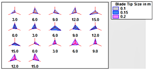
Figure 12 Sunray plot illustrating torque for blade tip sizes of 0.1, 0.15, and 0.2 m and blade twist angles of 0, 3, 6, 9, 12, and 15^∘ for three NACA airfoils.

Figure 13 Torque plot for NACA 0012, NACA 4412, and NACA 4415 airfoils.

4.1.1 Star glyphs and sunray plots for turbulence intensity

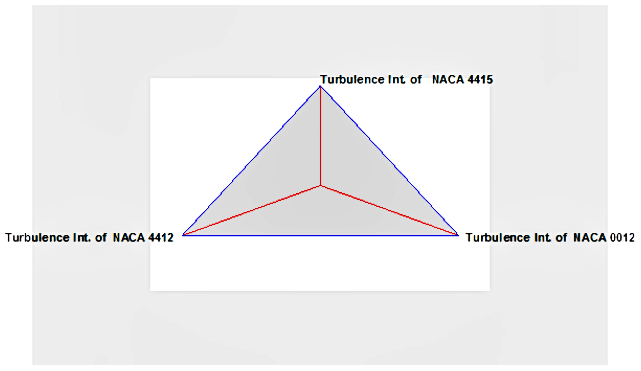
Based on the data mapping technique, different analysis and tasks are supported. Since we do not want to restrict ourselves in the analysis process, we aim for a design which supports both intra-record and inter-record comparisons. Data variables for the sample mean, standard deviation, and minimum and maximum values are provided in Table 2. From the identified data, the number of complete cases is recorded, and it is clear that NACA 4415 has appropriate output relating to the sample mean (2.19888), standard deviation (0.184452), the minimum value (2.01746), and the maximum value (2.78452). The sunray plot for blade twist angles of 0, 3, 6, 9, 12, and 15^∘ with a blade tip size of 0.1, 0.15, and 0.2 m is shown in Fig. 6. The star glyph is shown in Fig. 7 for NACA 0012, NACA 4412, and NACA 4415. The number of complete cases is 18.

Table 4 Data variables for vorticity.

The StatAdvisor for turbulence intensity

Figures 6 depicts the turbulence intensity of the three airfoils as the spokes of the sunray plots, and in Fig. 7, the star glyph displays the turbulence intensity of the three airfoils. In Fig. 6, three blade tip sizes (0.1, 0.15, and 0.2 m) and the blade twist angle are provided with each airfoil turbulence intensity reading. For the blade tip size of 0.1 and 0.15 m, the turbulence intensity is comparatively very low for all three airfoils, due to significant reduction of wind velocity behind the rotor for the upstream side compared with the downstream side. The turbulence intensity for all three airfoils with a 0.2 m blade tip size and a 9^∘ twist angle is observed as even, due to high mean wind speed created by means of wind tunnel wind flow well mixed with the flow of wind from the outer region of the wind tunnel. Minimum turbulence intensity is observed for the 0.1 blade tip size with a 3^∘ blade twist angle for airfoil NACA 0012.

Table 5 Data variables for torque.

The star glyph in Fig. 7 illustrates the turbulence intensity in the form of the geometric object that replicates each quantitative variable related to NACA 0012, NACA 4412, and NACA 4415.

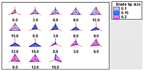
Figure 14 Normal force for blade tip sizes of 0.1, 0.15, and 0.2 m with blade twist angles of 0, 3, 6, 9, 12, and 15^∘ for three airfoils is shown.

Figure 15 Normal force representation for three NACA airfoils.

4.1.2 Star glyphs and sunray plots for static pressure

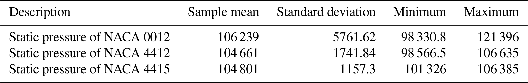
Data variables for static pressure revealing sample mean, standard deviation, and minimum and maximum values are provided in Table 3. For incoming air flow, the static pressure on the lower surface of the blade is more than the upper surface of the blade. As the pressure is lower on the upper surface, the incoming air will push the airfoil in the upward direction normal to the airflow. The number of complete cases is 18.

Table 6 List of data variables for normal force

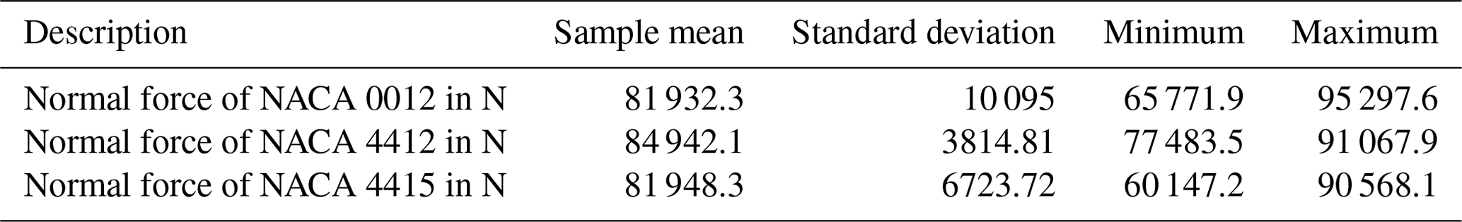
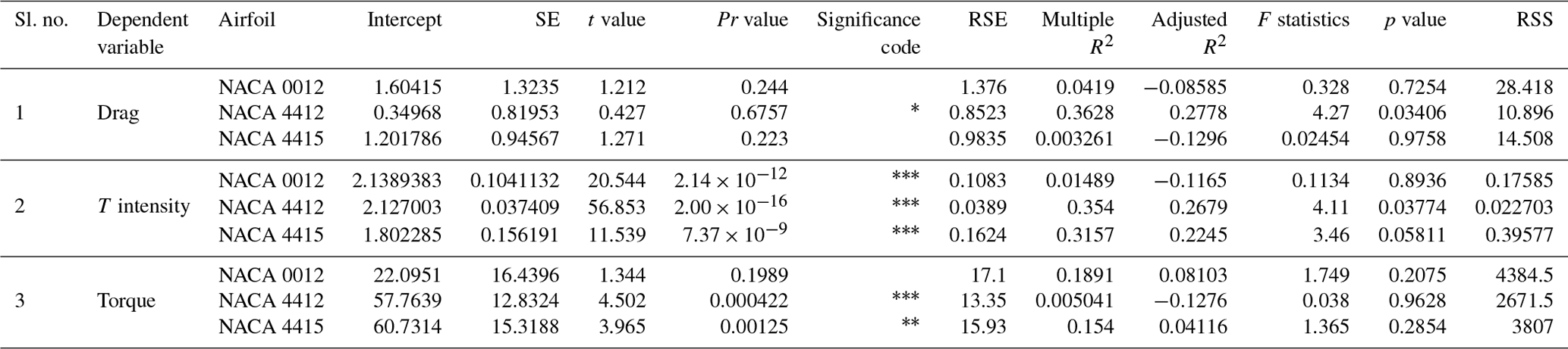
Table 7 Data generated from the R program for drag, turbulence intensity, and torque. RSS denotes the residual sum of squares; RSE denotes the relative standard error. Sl. no. is the serial number. The significance codes are shown as follows: ^* 0.01, ${}^{**}$ 0.001, ${}^{***}$ 0.

The StatAdvisor for static pressure

Figure 8 shows the static pressure for three NACA airfoils with blade twist angles of 0, 3, 6, 9, 12, and 15^∘ and blade tip sizes of 0.1, 0.15, and 0.2 m. From the sunray plot, it is clear that a blade tip size of 0.15 m with a blade twist angle of 12^∘ displays equal pressure acting on the free stream side of the airfoil, affecting the turbulence levels. Due to the higher drag and lift forces acting on the blade, a much lower static pressure is shown for a blade tip size of 0.1 and 0.2 m for a 0^∘ blade twist angle. The lowest static pressure is observed for the airfoil NACA 0012 with a 0^∘ blade twist angle and a 0.2 m blade tip size because of the symmetrical cross section of the airfoil in the suction side and the pressure side.

The star glyph and schematic representation of how data objects are mapped to the border region is depicted as shown in Fig. 9 for NACA 0012, NACA 4412, and NACA 4415. The star glyph displays static pressure in the form of the geometric object that replicates each quantitative variable related to the NACA 0012, NACA 4412, and NACA 4415.

4.1.3 Star glyphs and sunray plots for vorticity

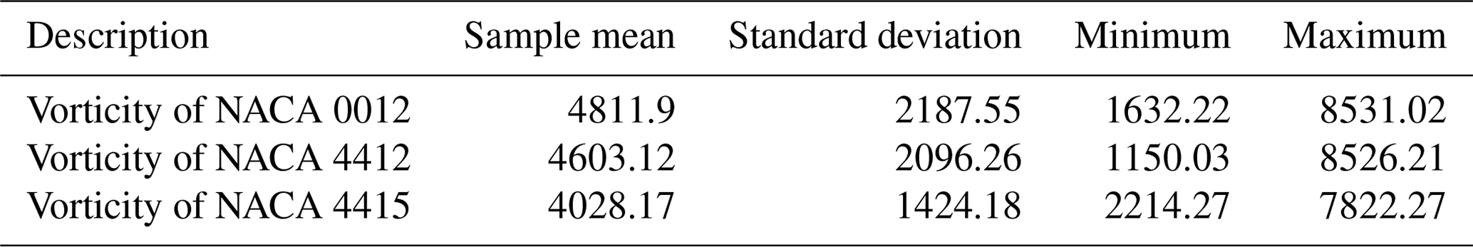
Data variables for vorticity revealing sample mean, standard deviation, and minimum and maximum values are provided in Table 4. From the identified data, the number of complete cases is recorded as shown below, and it is clear that, for each and every data, the value varies for NACA 0012, NACA 4412, and NACA 4415. Vorticity is defined as the circular motion of the wind, whereby the relative wind velocity is the key factor for vorticity. The number of complete cases is 18.

The StatAdvisor for vorticity

Figure 10 illustrates vorticities of three NACA airfoils with blade twist angles of 0, 3, 6, 9, 12, and 15^∘ and blade tip sizes of 0.1, 0.15, and 0.2 m. It is observed that the vorticity for the blade tip size of 0.1 m at a 0^∘ blade twist angle creates an appropriate plot for the three airfoils, as the vorticity is related to the mean wind speed when the rotor is high. At a 12^∘ blade twist angle, the highest vorticity is observed for NACA 4415. Similarly, the least vorticity is recorded for the 0.15 m blade tip size with a 12^∘ twist angle. The maximum and minimum vorticities are turbulence of the wind and non-periodicities of the downstream wind.

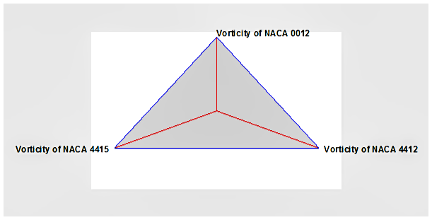
The star glyph is shown in Fig. 11 for three airfoils, NACA 0012, NACA 4412, and NACA 4415. The star glyph show the vorticity in the form of the geometric object that replicates each quantitative variable related to NACA 0012, NACA 4412, and NACA 4415.

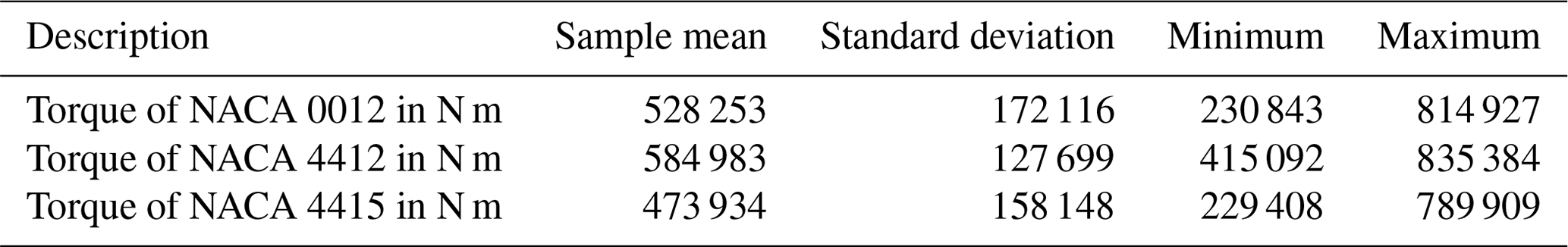
4.1.4 Star glyphs and sunray plots for torque

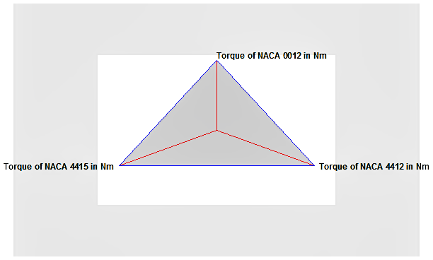
Data variables for torque revealing sample mean, standard deviation, and minimum and maximum values are provided in Table 5. From the identified data, the number of complete cases is recorded as shown below, and it is clear that, for each and every data, the value varies for NACA 0012, NACA 4412, and NACA 4415. The higher the torque, the higher the overall performance of the wind turbine. A close study of variables reveals that the maximum value of torque is obtained for NACA 0012. In an ideal fluid environment, the highest torque is attained when the drag coefficient is equal to zero. The number of complete cases is 17.

The StatAdvisor for torque

The sunray plot is shown in Fig. 12 for three NACA airfoils with blade twist angles of 0, 3, 6, 9, 12, and 15^∘ and blade tip sizes of 0.1, 0.15, and 0.2 m. Figure 12 demonstrates the torque for three airfoils. A consistent sunray plot is recorded for a 0.2 m blade tip size with a 6^∘ of blade twist angle. Hence, the wind energy is completely converted into useful energy, which leads to enhancement of wind turbine performance. For the blade tip sizes of 0.1 and 0.15 m, lower torque is observed at 3 and 12^∘ blade twist angles. Here, the lowest torque is observed for the airfoil NACA 4412. At this condition, the blade is ineffective in converting the wind energy to torque.

The star glyph in Fig. 13 displays torque in the form of the geometric object that replicates each quantitative variable related to airfoil NACA 0012, NACA 4412, and NACA 4415.

4.1.5 Star glyphs and sunray plots for normal force

Data variables for normal force revealing sample mean, standard deviation, and minimum and maximum values are provided in Table 6. From the identified data, the number of complete cases recorded is shown below, and it is clear that, for each and every data, the value varies for the three airfoils NACA 0012, NACA 4412, and NACA 4415. The number of complete cases is 18.

The StatAdvisor for normal force

Figure 14 shows that an appropriate graphical analytic plot is recorded for the 0.1 m blade tip size with a 15^∘ blade twist angle for the three airfoils. Normal force depends on the wind shear conditions and aerodynamic forces along the blade and rotor. Due to much stronger wind shear and high aerodynamic forces, for blade tip sizes of 0.15 and 0.2 m, lower normal force is observed for a blade tip size with a 0^∘ blade twist angle for the airfoil NACA 4412. Minimum normal force is observed for the airfoil NACA 4415 with a blade tip size of 0.2 m and a blade twist angle of 15^∘.

The star glyph is shown in Fig. 15 for NACA 0012, NACA 4412, and NACA 4415. The star glyph (triangle shape) displays normal force in the form of the geometric object that replicates each quantitative variable related to NACA 0012, NACA 4412, and NACA 4415.

4.2 Multilinear regression analysis

The simulation data are analysed using the multilinear regression R program for data visualization. Table 7 displays the multilinear regression analysis output obtained in the R program. Here data normalization is done for the dependent variables torque, static pressure, dynamic pressure, and relative pressure of 10⁻⁴ and vorticity normal force of 10⁻³ to control and interpret the data values.

4.2.1 Drag

From Table 7, for all three airfoils, dependent variable drag is less significant, and the R² value is close to zero, which shows that the model is not fit. As the p value is less than zero, the null hypothesis is rejected. RSE predicts the measure of error. A lower value of RSE enhances the accuracy of the model. Here, the RSE is less than zero for all three airfoils.

A drag scatter plot is shown in Fig. 16, with drag as the dependent variable for the blade twist angle and blade tip size of three airfoils. For airfoils NACA 0012 and NACA 4412, there is a least correlation between the independent variables angle and tip, as the points are distributed randomly. This is highlighted by the blue-coloured oval shape. It is observed that the random distribution of scatter points is high for the independent variable angle in the case of all three NACA airfoils. Similarly, for the independent variable tip, the scatter points are randomly distributed only for two airfoils, NACA 0012 and NACA 4415. The scatter points' distribution is in good agreement with the tip for the airfoil NACA 4415, as shown by the green-coloured oval shape. The drag depends on the air movement passing through the airfoil and is largely dependent on the geometry of the blade. Hence, the drag for the airfoil NACA 4415 is strongly correlated as the scatter points are linear with respect to blade tip size, and the model leads to better estimation of the drag variable with regression analysis.

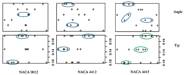
Figure 16 Three airfoils NACA 0012, NACA 4412, and NACA 4415 and the scatter plot for drag are considered for blade tip size and blade twist angle.

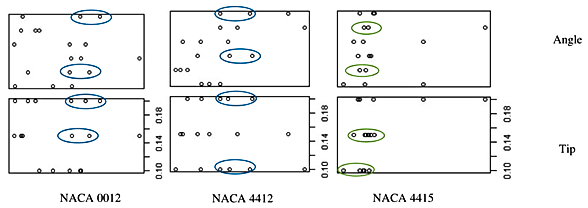
Figure 17 Turbulence intensity scatter plot for blade angle and blade tip size of airfoils NACA 0012, NACA 4412, and NACA 4415.

4.2.2 Turbulence intensity

Figure 17 illustrates the scatter plot of turbulence intensity variable for three airfoils NACA 0012, NACA 4412, and NACA 4415 on the x axis and y axis, with the angle and tip in the first and second rows respectively. By looking at the scatter plot, it is clear that there is a least correlation between the angle and airfoils NACA 0012 and NACA 4412 as the scatter points are randomly distributed. For the independent variable tip, there is a possibility of linear correlation as the scatter points are linearly fit. Also, it is considered that turbulence intensity is fit for the model for all three airfoils. However, the possibility of linear fit for the angle and tip is observed with the airfoil NACA 4415. This reflects that the dependent variable turbulence intensity is strongly correlated with airfoil NACA 4415 and shows that the NACA 4415 airfoil enhances the performance of the wind turbine. However, for the airfoil NACA 4415, the scatter points are closer at the blade tip size of 0.14 to 0.18. This states that correlation exists between the airfoil NACA 4415 and blade tip size. It also suggests that the airfoil NACA 4415 has the best linear fit. The green-coloured oval shape depicts the linear fit model, whereas the blue-coloured oval shape illustrates the randomly distributed turbulence intensity scatter points.

From Table 7, it is clear that there is high significance for all three airfoils. The null hypothesis is rejected as the p value is lower than zero for all three airfoils. The model is found to be accurate as the RSE value is lower than zero. The RSE is said to be the measure of error prediction. Based on analysis of variance, the residual sum of squares is less than zero for all three airfoils, which means that there is a linear fit in the model for the given data.

4.2.3 Torque

The scatter plot in Fig. 18 shows that the scatter points of torque in angle are randomly distributed with the blade twist angle for airfoils NACA 0012, NACA 4412, and NACA 4415, and there is no strong correlation between them, as shown in the coloured lines. In the case of blade tip size, the torque scatter points are linearly distributed for the value 0.14 for two airfoils, NACA 4412 and NACA 4415, respectively as shown by the green-coloured oval shape, which shows that the torque generated is adequate to improve the wind turbine performance.

Table 8 The coefficients of dependent variables lift, normal force, and vorticity. The significance codes are shown as follows: ${}^{**}$ 0.001, ${}^{***}$ 0.

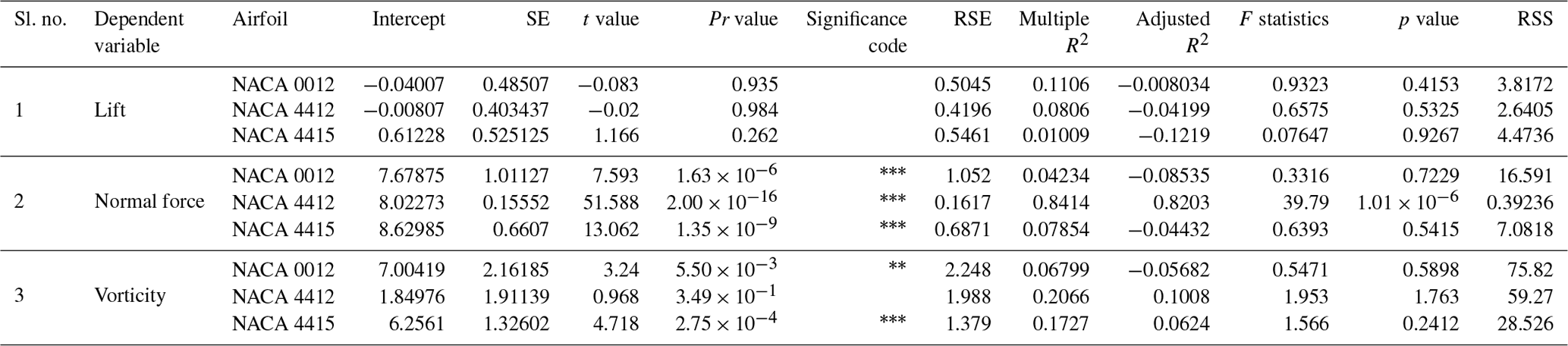
Table 7 gives the intercept β value, standard deviation, t value, Pr value, significance code, R² value, and so on. As we notice that the p value is low (for airfoils NACA 0012 and NACA 4415) and close to 1 (for NACA 4412), it means that the coefficient is significant. For lower p values, the null hypothesis is rejected. For the torque, the residual sum of squares is higher (for airfoil NACA 0012, it is 4384.5), and the model does not fit the data.

Figure 18 Scatter plot of torque with blade angle and blade tip size of three airfoils.

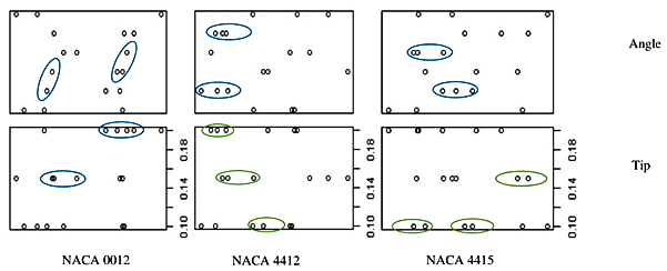
Table 8 displays the three performance parameters lift, normal force, and vorticity and the coefficients generated using the R program with three airfoils NACA 0012, NACA 4412, and NACA 4415.

4.2.4 Lift

From Table 8, dependent variable lift is less significant for all three airfoils, and the R² value is less than zero, which states that the model is not fit. As the p value is less than zero, the null hypothesis is rejected. RSE predicts the measure of error, and the lower values of RSE enhance the accuracy of the model. Here, the RSE is less than zero for all three airfoils.

Lift is taken as the dependent variable; the independent variables taken are blade twist angle and blade tip size, and individual airfoils considered are NACA 0012, NACA 4412, and NACA 4415 as shown in Fig. 19. The lift scatter plot for the angle (highlighted by the blue-coloured oval shape) is randomly distributed on the x axis for three airfoils, which shows that the lift coefficient is inadequate for the independent variable blade angle. For the y axis, the tip in the second is in good correlation as the points are linearly distributed (represented by the green-coloured oval shape) for the three airfoils NACA 0012, NACA 4412, and NACA 4415, which means the blade tip size is effective in evaluating the wind turbine efficiency.

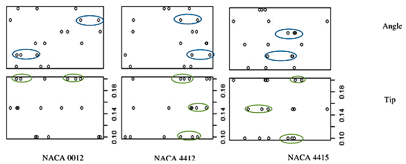
Figure 19 Scatter plot of lift for blade angle and blade tip size of airfoils NACA 0012, NACA 4412, and NACA 4415.

4.2.5 Normal force

Figure 20 illustrates the scatter plot of normal force variable for three airfoils NACA 0012, NACA 4415, and NACA 4415 on the x axis and y axis, with the angle and tip in the first and second rows. By looking at the plot, it is clear that there is a least correlation between the scatter points which are randomly distributed for all the NACA 0012 airfoils with the y axis independent variable angle. For the case of airfoil NACA 4412 and NACA 4415, the normal force scatter points are least randomly distributed and stated as linearly fit. In other words, the blade angle is adequate for the wind speed of 36 m s⁻¹ for the airfoil NACA 4412 and NACA 4415. However, an independent variable tip only makes a significant linear model for the airfoil NACA 4412. The linearly distributed points are highlighted by the green-coloured oval shape and blue-coloured oval shape, which represent randomly distributed points.

From Table 8, it is seen that there is high significance for all three airfoils. The null hypothesis is rejected as the p value is lower than zero for all three airfoils. The model is found to be accurate as the RSE value is lower than zero for the airfoils NACA 4412 and NACA 4415. The RSE is said to be the measure of error prediction. Based on analysis of variance, the residual sum of squares is less than zero for the airfoil NACA 4412, which means that there is a linear fit in the model for the given data.

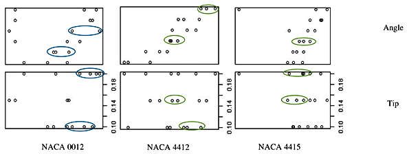
Figure 20 Normal force scatter plot for blade angle and blade tip size of airfoils NACA 0012, NACA 4412, and NACA 4415.

4.2.6 Vorticity

The scatter plots in Fig. 21 are randomly distributed, and the outliers are in large number, as shown by the ovals. This shows that the three airfoils are not highly correlated with the angle. By considering the tip, the vorticity variables are linearly adequate for the NACA 0012, NACA 4412, and NACA 4415 airfoils, given by the green oval shapes. It means adequate wind is generated to rotate the rotor with different values of vorticity. Table 8 records the β value, standard deviation, t value, Pr value, significance code, R² value, and so on. As we notice that the p value is low (for airfoil NACA 0012 and NACA 4415) and close to 1 (for NACA 4412), it means the coefficient is significant. For lower p values, the null hypothesis is rejected. For the torque, the residual sum of squares is higher (for airfoil NACA 0012 is 4384.5), and the model does not fit the data.

Figure 21 Dependent variables with list of coefficients for three airfoils.

The coefficients of dependent variables dynamic pressure (pressure D), relative pressure (pressure R), static pressure (pressure S), total pressure (pressure T), and axial velocity (velocity A) are listed in Table 7. The coefficients are determined for each NACA airfoil using the R program.

Table 9 Dependent variables with list of coefficients for three airfoils.

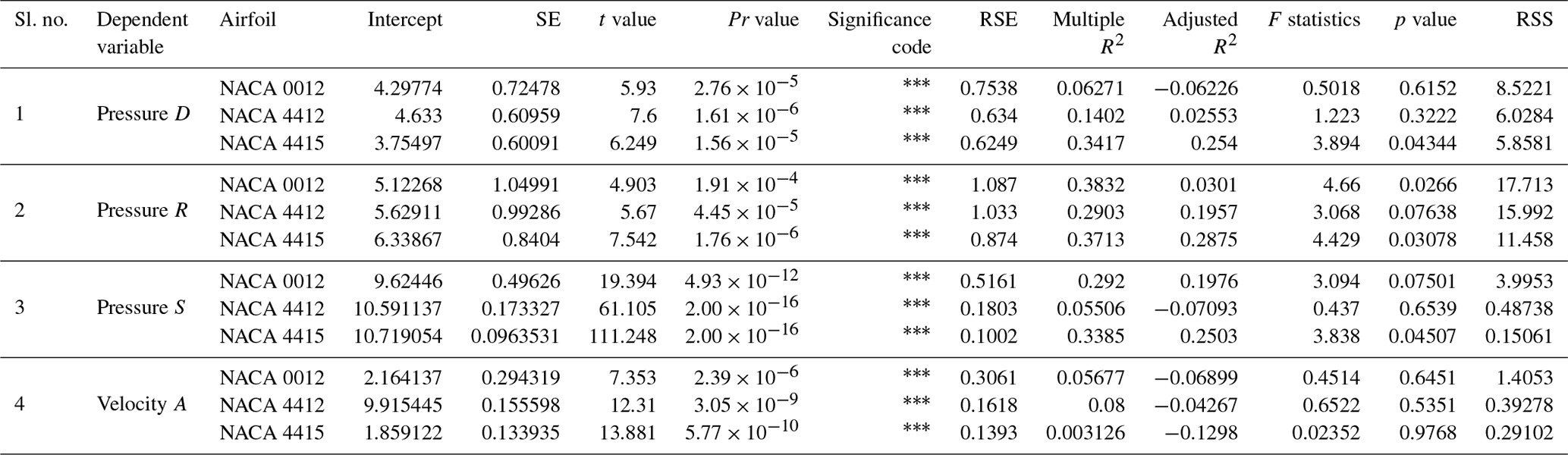
4.2.7 Dynamic pressure

From Table 9, for all three airfoils, it is observed that the dependent variable dynamic pressure is highly significant, and the R² value is less than zero, which shows that the model is not fit. The intercept values are 4.29, 4.633, and 3.75 for the airfoils NACA 0012, NACA 4412, and NACA 4415 respectively, based on the multilinear regression analysis. As the p value is less than zero, the null hypothesis is rejected.

Dynamic pressure is taken as the dependent variable, and the independent variables taken are blade twist angle and blade tip size. Individual airfoils considered are NACA 0012, NACA 4412, and NACA 4415, as shown in Fig. 22. For the airfoil NACA 0012, the dynamic pressure scatter plot is randomly distributed (represented by the blue-coloured oval shape at scatter points) and not linearly fit, which states that the formation of dynamic pressure is not strong with respect to blade angle and blade twist. However, for the airfoil NACA 4412 and NACA 4415, there is a linear relationship (as the points are closely distributed – highlighted by the green-coloured oval shape) for the dynamic pressure points between the angle and tip. Also, an adequate amount of dynamic pressure is generated to start the wind turbine.

Figure 22 Scatter plot matrices for blade angle and blade tip size of three NACA airfoils.

4.2.8 Relative pressure

Figure 23 illustrates the scatter plot of relative pressure variable for three airfoils NACA 0012, NACA 4415, and NACA 4415 on the x axis and y axis, with the angle and tip in first and second rows. The relative pressure scatter points in the independent variable angle are randomly distributed for the three airfoils. This shows that the independent variable angle is not linearly fit (highlighted by the blue-coloured oval shape), and there is no strong relation between them. The independent variable in the second row of the y axis (tip) seems to be linearly fit as the scatter points in the three airfoils are close (highlighted by the green-coloured oval shape).

From Table 9, it is seen that there is high significance for all three airfoils. The null hypothesis is rejected as the p value is lower than zero for all three airfoils. The model is found to be accurate as the RSE value is lower than zero for the airfoils NACA 4412 and NACA 4415. The RSE is said to be the measure of error prediction. Based on analysis of variance, the residual sum of squares is less than zero for the airfoil NACA 4412, which means that there is a linear fit in the model for the given data.

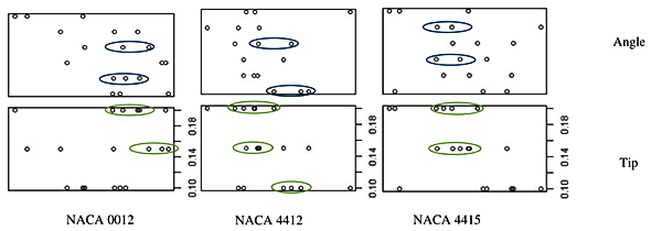
Figure 23 Scatter plot for blade angle and blade tip size of airfoils NACA 0012, NACA 4412, and NACA 4415.

4.2.9 Static pressure

Static pressure scatter points are shown in Fig. 24, in which the points are close to each other and linearly fit for three airfoils NACA 0012, NACA 4412, and NACA 4415 for both the independent variable angles, as shown by the green oval shape. For the airfoils NACA 0012 and NACA 4412, the scatter points are only randomly distributed with the tip, represented by the blue-coloured oval shape. Hence, it is clear that the relative pressure for the airfoils NACA 0012 and NACA 4412 is low with the blade tip size when compared with the angle and tip of airfoil NACA 4415.

Table 9 depicts the correlations from the R program, in which strong significance exists for three airfoils. The negative adjusted R² value means the static pressure is less than the atmospheric pressure. The residual sum of squares is 1, which means the model is strongly correlated, and there is a linear relationship.

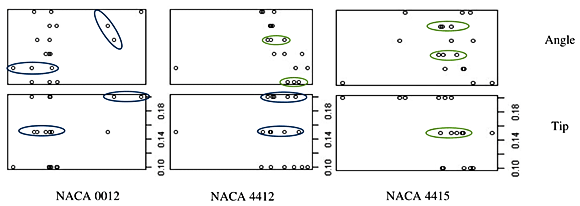
Figure 24 Static pressure scatter plot for blade angle and blade tip size of airfoils NACA 0012, NACA 4412, and NACA 4415.

4.2.10 Axial velocity

The coefficients in Table 9 have good significance for the three airfoils as the Pr value is less than zero. The RSE is less than zero, which is the measure of error prediction and defines the model is fit. However, the null hypothesis is rejected for the airfoils NACA 0012 and NACA 4415 as the p value is less than zero.

Figure 25 displays the scatter plot of axial velocity for three airfoils NACA 0012, NACA 4412, and NACA 4415 with respect to the y axis angle of the blade and tip of the blade. The airfoils NACA 0012 and NACA 4412 are said to be linearly fit for the angle and tip as the axial velocity scatter points are closely distributed (highlighted by the green-coloured oval shape). This shows that the axial velocity for the NACA 0012 and NACA 4412 is closer and sufficient axial velocity is generated to rotate the rotor. For the airfoil NACA 4415, the linear fit does not only exist for the independent variables' angle and tip.The scatter points are randomly distributed (highlighted by the blue-coloured oval shape), and it can be said that the axial velocity does not have a strong correlation with the airfoil NACA 4415.

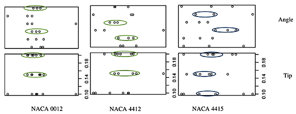
Figure 25 Three independent variables determine the axial velocity in the form of a scatter plot.

5 Conclusions

The approach in this research includes data visualization and multilinear regression analysis. Multiple linear regression is a standard selection model in the world of data science. In this model, the prediction of models is based on the data from the design and analysis of horizontal axis wind turbines. These obtained data are assigned to R programming with empirical correlations. The approach turned to be promising. However, the results reveal that the implemented technique holds a high degree of predictions, and the number of data sets is adequate. It is also observed that errors are in less concentration as the sum of squared errors is zero for every parameter. The following conclusions are made.

• The turbulence model is considered and validated with the boundary layer mesh along with numerical equations.

• Based on the data visualization technique, standard deviation, sample mean, and minimum and maximum values for the three airfoils for six different blade twist angles and three blade tip sizes, NACA 4415 provides validated results in comparison with NACA 0012 and NACA 4412. It is found that the geometric object replicates each quantitative variable.

• Finally, the statistical analysis discusses the influence of the blade angle and blade tip size and three airfoils as independent variables, with dependent variables drag, lift, normal force, static pressure, dynamic pressure, relative pressure, turbulence intensity, torque, axial velocity, and vorticity. From the multilinear regression analysis, the parameters drag and lift are less significant, and the torque, normal force, relative pressure, static pressure, dynamic pressure, turbulence intensity, axial velocity, and vorticity are highly significant as the p value is less than 0.

• From performance analysis and by comparing overall results, the airfoil NACA 4415 looks to be a good fit. It maximizes the power output from the wind turbine model and also enhances the efficiency of the wind power plant. This airfoil NACA 4415 will be suitable to install in the next generation of renewable energy wind power stations.

• Further, the multilinear regression model combined with a multi-nominal logistic regression model is a great approach for the prediction of trends of electricity generation from horizontal axis wind turbines based on rotor blade and hub analysis.