the Creative Commons Attribution 4.0 License.
the Creative Commons Attribution 4.0 License.
 | 03 Jun 2020
Dynamic parameters identification of a haptic interface for a helicopter flight simulator
Dingxuan Zhao
Jianyao Zhang
Giuseppe Carbone
Haojie Yang
Tao Ni
Shuangji Yao
The haptic interface force feedback is one of the key factors for a reliable flight simulation. This paper addresses the design and control implementation of a simple joystick-like haptic interface to be used for a helicopter flight simulator. The expression of the haptic interface force is obtained by dynamic analysis of the haptic interface operation. This paper proposes a new strategy aiming at avoiding the use of an expansive and complex force/torque sensor. Accordingly, specific dynamic model is implemented by including Stribeck friction to describe the friction moment. Experimental data are processed as based on a genetic algorithm for identifying the dynamic parameters in the Stribeck friction model. This allows to obtain the friction moment parameters of the haptic interface, as well as the torque distribution due to gravity and the rotational inertia parameters of the haptic interface for the calculation of the haptic interface force. Experimental tests are carried out and results are used to validate the proposed dynamic model and dynamic parameter identification method and demonstrate the effectiveness of the proposed force feedback while using a cheap photoelectric sensor instead of an expansive force/torque sensor.
- Article
(2805 KB) - Full-text XML
- BibTeX
- EndNote


Due to the high risks and costs of training on a real helicopter, pilots often need to complete a preliminary training on a helicopter flight simulator. Real flight training is carried out only after a successful training on a simulator. In helicopter flight simulators, the joystick is a key element, which is used to achieving a reliable helicopter driving while providing a force feedback feeling, which needs to properly mimic the force feedback feelings of a real helicopter flying (Prachyabrued and Robert, 2018). In the real flight control process, the pilot's hand will feel the feedback force and make judgments, then adjust the flight status through the feedback force. In the whole process, the current force of the haptic interface needs to be used as the simulation calculation of the feedback force. Thus, its measurement accuracy is particularly important. Most of the operating forces are measured by using torque sensors. The papers Cavallo et al. (2004), Rinaldi and Beckham (1983), Hutton et al. (1994), and Fergani et al. (2016) installed a pull-up/pressure sensor at the end of the rod to read the applied force at each moment. However, torque sensor occupies large space in both mechanical installation and wiring, which affects the normal operation of the pilots. This paper proposes a different strategy aiming at avoiding the use of an expansive and complex force/torque sensor. Namely, the proposed approach is based on establishing a reliable dynamic model of the haptic interface to replace the role of the force/torque sensor. Accordingly, a proper dynamic model and a parameter identification strategy have been proposed.
In a servo system, there are complex rolling friction and sliding friction phenomena between gear train, bearing, input/output shaft and seal. Therefore, the modelling of friction torque is very important, which directly affects the dynamic accuracy of the haptic interface. A variety of empirical models have been proposed for friction calculation of servo system, which can be divided into two phases: static friction model and dynamic friction model (Bona and Indri, 2005). The most widely used static friction model is the Stribeck model. Several papers analyzed the friction of a servo system by establishing its Stribeck friction model (Lichun and Pavelescu, 1982; Xu et al., 2011; Chen et al., 2016; Márton and Lantos, 2009; Broel-Plater et al., 2018). Considering the advantages and drawbacks of the existing models in literature, it has been decided to implement a Lugre model to analyze the friction of the servo system, as proposed in Canudas de Wit et al. (1995), Wang et al. (2019), Azizi and Yazdizadeh (2019), Freidovich et al. (2010), and Ishikawa et al. (2010). Main advantage of Lugre model is its relatively high accuracy, while its implementation is relatively complex, since it introduces an unknown quantity which can be difficult to be measured directly and requires a high precision servo system. The Stribeck model is currently used in many fields to model the friction moment. Since there are unknown parameters in the haptic interface dynamics model, such as gravity moment, Stribeck friction moment model parameters and rotational inertia, these parameters need to be identified. The main available parameter identification methods are tracing methods, least square methods, and genetic algorithms. The genetic algorithms are very effective evolutionary random search methods, which are proven in literature to be very effective in managing non-linear problems with a high level of computational robustness and calculation parallelization. Accordingly, genetic algorithms can be seen as the most convenient approach for addressing this identification problem. In this paper, a dynamic analysis is carried out on the a 2-dof flight haptic interface for a helicopter simulator. A nonlinear Stribeck model is established for the friction torque of the servo system. A curve fitting and genetic algorithm method are used for processing the data to identify the gravity torque, four parameters of the Stribeck model and the rotational inertia. Finally, the available parameters identified are brought into the dynamic model to calculate the haptic interface force in real time and an experimental validation is carried out to proof the effectiveness of the proposed approach.
2.1 The proposed haptic interface and its operating principles
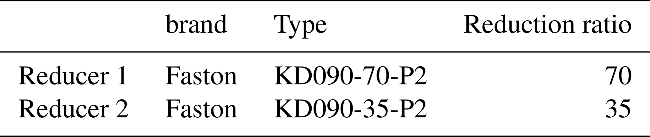
This paper adopts the helicopter simulator at laboratory in Yanshan University which is shown in Fig. 1. The helicopter flight simulator is mainly composed of four modules: a helicopter simulation cockpit system, a virtual scene system, a dynamic motion system and an audio system. The simulator's haptic interface is shown in Fig. 2. The haptic interface is driven by two servomotors, and two disc speed reducers are used for speed regulation. The motor adopts Kollmorge CKM04 AC permanent magnet synchronous servo motors, and its corresponding AKD series servo driver supports Modubus TCP communication. The parameters of the servo motors and the reducers are shown in Tables 1 and 2. The hardware system composition of the haptic interface is shown in Fig. 3.
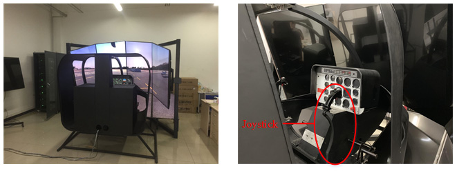
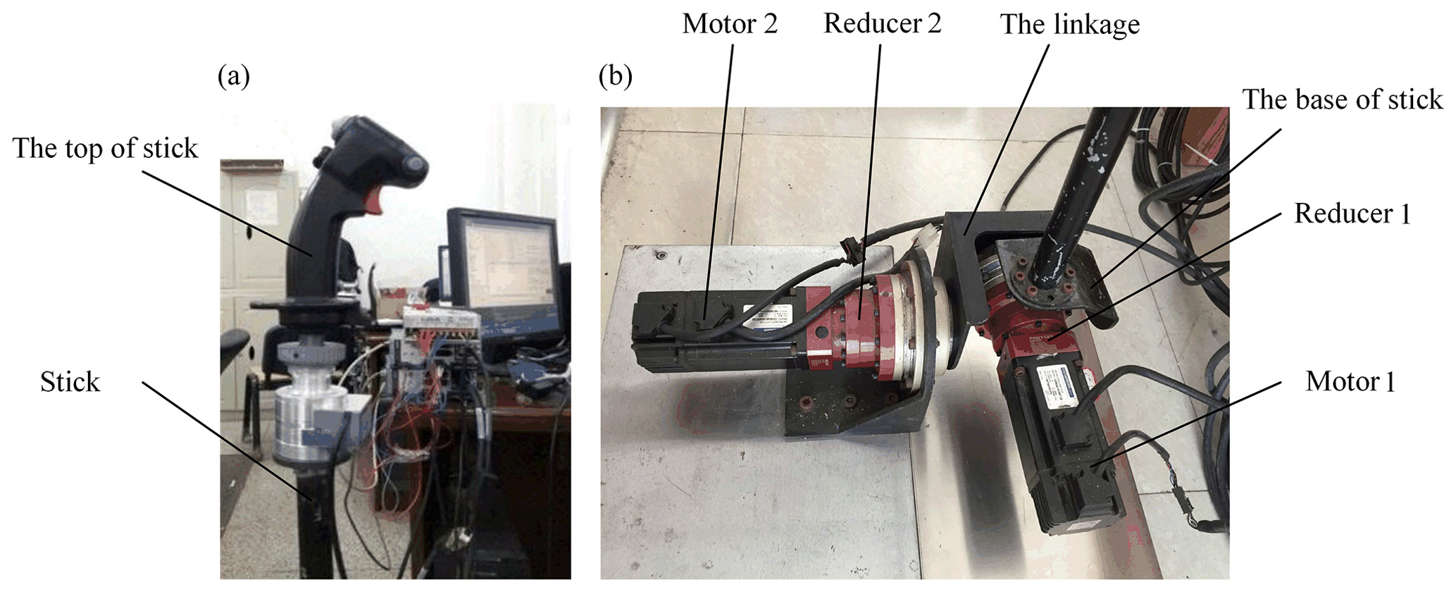
Figure 2Force feedback test bench of haptic interface. (a) Control handle; (b) servo motor and rotating mechanism.

First, the computer is connected to the switch, and the switch is connected with two motor drivers respectively through Enternet port. Then, C programmed code has been written to establish communication between servo motor and computer through Modbus TCP protocol. When the driver operates the haptic interface, the computer can obtain the current electricity value from the servo motor at each time. Then, the driving torque of the servo motor is obtained. At the same time, the photoelectric encoder of the servo motor can measure the stick's position and speed at the current time, which can be used for the dynamic calculation of the haptic interface.

2.2 Dynamic analysis of the haptic interface
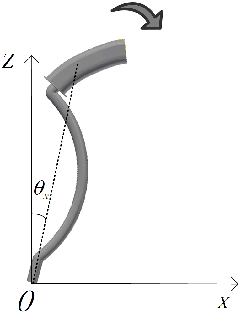
First, coordinate system for the haptic interface is established for the haptic interface, as shown in Fig. 4. The intersection point of the two motor axes is defined as origin O. The two motor axes are set as x axis and y axis respectively. z axis is perpendicular to the xy plane.

The free-body diagram is shown in Fig. 5. The angle θ, θx, θy formed between the haptic interface and the z axis is the output angle of reducer 1 and reducer 2 respectively. the relationship of the three parameters can be expressed as follows:
When the haptic interface moves, the control handle, the haptic interface and the base of the haptic interface move at an angle θ, the motor 1, the reducer 1 and the rotating mechanism move at an angle θy.
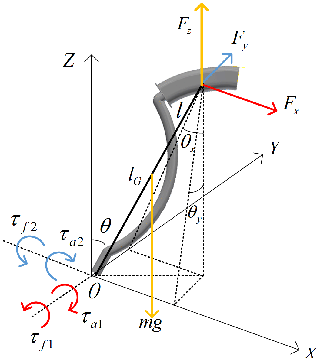
In Fig. 5, m is the mass of the haptic interface system, lG is the distance between the center of mass of the haptic interface and the origin, and l is the distance between the top of the stick and the origin. τa1 and τa2 are the output torques by motor 1 and 2 through the disc reducer respectively; τf1 and τf2 are the friction torques on the x axis and y axis of the servo system respectively. The manual force of the pilot in the direction of x axis, y axis and z axis defined as Fx, Fy, Fz.
The Lagrange method is adopted to conduct dynamic analysis of the system. The Lagrange function can be formulated as
In Eq. (2), Ek is the kinetic energy of the haptic interface system; Ep is the potential energy of the haptic interface system; , in the haptic interface system represent the output angles θx, θy of the two reducers respectively.
The total kinetic energy Ek for the haptic interface system can be expressed as:
In Eq. (3), J1 is the sum of the moment of inertia of motor 1, reducer 1 and rotating mechanism; J2 is the sum of the moment of inertia of the control handle, haptic interface and haptic interface base.
The potential energy of the haptic interface Ep can be expressed as:
In combination with Fig. 5 and Eq. (1), the following equation can be obtained:
According to the comprehensive Eqs. (2)–(5), can be obtained:
In Eq. (6), τ1 and τ2 are the torques exerted by the pilot on the x axis and y axis during the control process respectively.
Especially, the torque output τa by the motor through the disc reducer is related to the reduction ratio i of the reducer and the output torque Ta of the motor, as:
Ta can be deduced from Eq. (7):
In Eq. (8), Pn is polar logarithm; ψr is the flux chain of rotor magnetic pole; Ld, Lq is the armature inductance of axis d and axis q; Id, Iq is the current of d axis and q axis.
Since the armature inductance of d axis and q axis of the motor used same value, namely:
From Eqs. (7), (8) and (9) can be obtained as follows:
At this time, the torque and the q axis current have a linear relationship, which can be expressed as:
Combined with Eqs. (6) and (11), and using mglG replaced by the gravity moment TG, the following equation can be obtained:
Thus, the manual force of the pilot can be expressed as:
2.3 Friction torque model of the haptic interface
In the haptic interface structure, there are complex frictions within the servo motor and between the reducer. The friction torque generated by these frictions has a great influence on the accurate modelling of the haptic interface. Therefore, the friction torque at each moment must be accurately obtained to ensure the accuracy of the calculated force and torque at each moment.
The classic Coulomb friction model friction indicated that friction force is related to the positive pressure acting on the object. However, due to the lubrication in the servo system, the influence of viscous friction must be considered.
Stribeck proposed to model the servo friction as a combination of Coulomb friction and viscous friction. He has given a quantitative formulation for friction with respect to velocity (Balogh and Krstic, 2004). Similarly, the Stribeck formula can be converted into the formula of friction torque regarding motor speed as proposed in (Iwasaki et al., 1999):
In Eq. (14), ω is the motor speed; τc is Coulomb friction torque; τs is the maximum static friction torque; ωs is Stribeck speed; Bω is the coefficient of viscous friction.
The Stribeck curve is related to the speed of the servo system. In the low-speed area, it is affected by Coulomb friction and viscous friction, and the friction torque decreases. This area is called boundary lubrication friction area. With the increase of speed, the influence of viscous friction is much higher than Coulomb friction. At this time, the friction torque is approximately proportional to the rotational speed. This operation condition is defined as liquid lubrication condition.
There are two problems in applying the Stribeck friction model to the control of haptic interface force control: on the one hand, it is difficult to describe the change of haptic interface friction torque when the velocity is zero; on the other hand, the change of velocity near the zero point will cause a sudden change of friction torque, which will lead to a jitter in the reversing process. Therefore, approximate treatment of the low speed phase of the Stribeck friction model is required. This paper proposes to use a sigmoid function to deal with Stribeck friction model (Ciliza and Tomizuka, 2007).
The Stribeck friction torque model improved by sigmoid function can be expressed as follows:
According to the requirements of the model and accuracy, the value of γ is defined as 500 in the proposed model.
3.1 Identification of the gravity torque model parameter
According to Eq. (13), the total force applied to the haptic interface is directly related to the magnitude of the gravity torque TG. In order to obtain an accurate model, it is necessary to identify the gravity torque TG. This is achieved with an experiment conducted on the motor 1 when its movement is on xz plane. Set the haptic interface to rotate at a constant speed, and then is zero. The haptic interface was not moved in the y direction, so θy is zero. The driver has no additional force to the haptic interface, accordingly also τ2 is zero. Since the velocity is constant, τf1 is constant. In addition, sin θx is relatively small in practical application, accordingly θx can be used instead. The experimental process is shown in Fig. 6 and Eq. (6) can be converted into:
At this time, θx maintain a liner relationship with Iq1 have a linear relationship. Discretizing Eq. (16) one can obtain:
A following experiment consists in setting the motor speed at 40 rpm (Rotation per minute), make the haptic interface rotate at a constant speed, take the values of θx and Iq1 in multiple groups. A curve fitting of the results in such experiments is shown in Fig. 7. The identified gravity torque is 11.14 N m. The toolbox of Curve Fitting Tool in Matlab is used to get the result.

3.2 Identification of friction torque model parameters via genetic algorithm
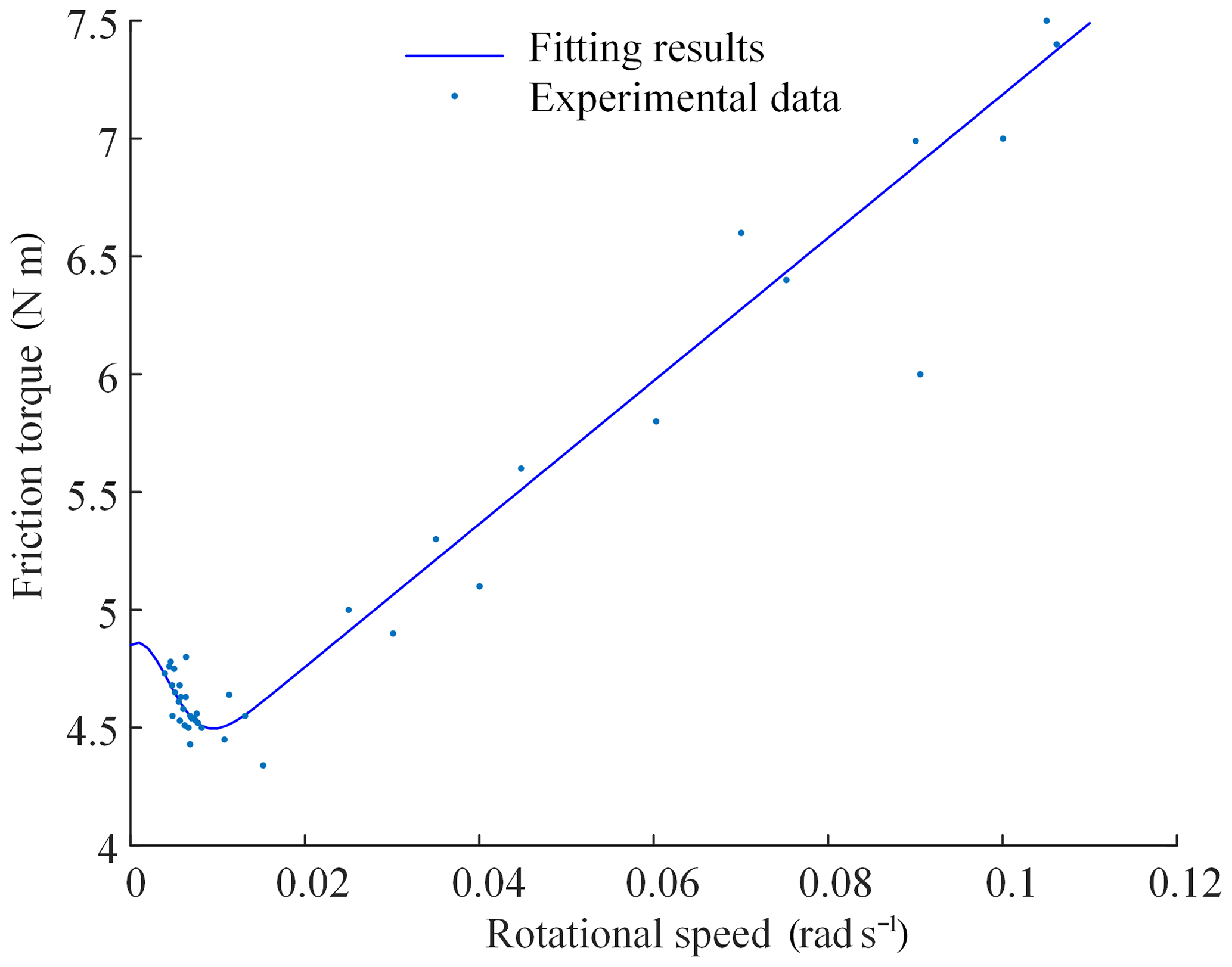
When we choose Stribeck friction model, it contains four unknowns: τc, τs, ωs and Bω, these four parameters need to be identified. Similarly, the motor 1 is set as the speed mode and a specific motor speed is given to make the haptic interface rotate at a constant speed. At the same time the driver has no additional force to the haptic interface, in this case, θy, and τ1 are equal to zero. Therefore, according to Eq. (6), the following equation can be obtained:
According to Sect. 2.1, the current value, rotation angle and rotation speed of the motor can be read at each moment. It is can be concluded from Eq. (18), the friction torque τf1 at the corresponding rotational speed can be obtained. The value of friction torque τf1 can be obtained by the different output angle .
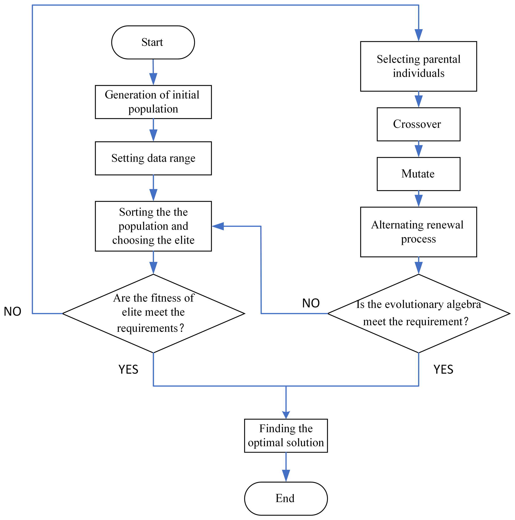
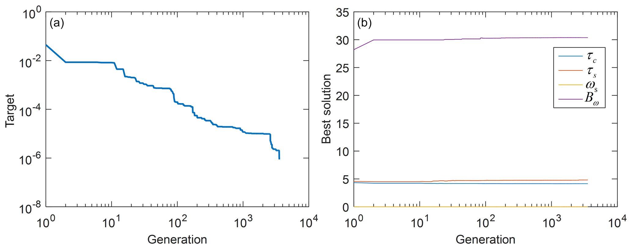
Figure 9Parameter identification process of friction model. (a) The objective function changes with generations; (b) the elite individual changes with generations.
Genetic algorithm is an algorithm designed according to Darwinian evolution theory: through continuous natural selection, survival of the fittest, so as to obtain the most adaptable results (Liu, 2006). The process of parameter identification mainly includes generation of initial population, selection of race parameters, setting of fitness function, selection, crossover, variation and termination.
The search scope of parameters τc, τs, ωs and Bω can obtained by tracing method. The iteration interval is [4–5], [4–5], [0–0.1] and [20–40] respectively. The population size was set as 100, and the crossover probability and mutation probability were set as 0.4 and 0.1 respectively. The selection of GA parameters has been carried out by considering the peculiarities of the specific identification problem as well as several preliminary identification tests. In particular, after preliminary identification tests we selected 0.4 as crossover parameter and 0.1 as variation parameters. The selected crossover parameter gives a preference to parental individuals on filial individuals. The selected variation value is motivated by a limited influence of variation on this specific parameter identification. Numerical simulations have been carried out also with other values of the crossover parameter (e.g. 0.4 and 0.8). Results led to similar outcomes of the identification procedure.
The multi-group friction torques obtained through Eq. (18) can be expressed as:
In Eq. (8), , , and are the four parameters to be identified respectively, and is the theoretical friction torque calculated by the motor speed. Take the target function:
The actual identification task of genetic algorithm is to solve the minimum value of objective function.
The minimum target value is defined as 10−6 here, and the maximum evolutionary algebra is 10 000 generations. In each generation, the population is sorted in ascending fitness order, and the optimal solution of this generation is recorded as the elite. Parental individuals were selected in the fitness sequence for crossover, and the offspring were mutated. Finally, when the fitness of a certain generation of elite meets the requirements () or the evolutionary algebra is more than 10 000 generations, the whole selection process of genetic algorithm is terminated.
The process of genetic algorithm is shown in Fig. 8, and its identification process is shown in Fig. 9. Figure 10 shows the comparison between the theoretical friction moment calculated by the identified parameters and the actual friction moment. The measurement result of the friction torque at the moment of is the same as the moment of , but the symbol is opposite, so it was omitted. Here we only figure out the absolute value of the friction torque. The identified parameters at the end of program operation are shown in Table 1. The identification of friction model parameters in the y axis direction was the same as that in the x axis. The identification results are listed in Table 3. Several cases have been considered in the identification process for the friction torque model parameters to obtain a reliable mean value of all the parameters. Considering the characteristics of the proposed identification process we can estimate a confidence interval of 0.0001 % (the minimum target value is in Eq. 20), which can be considered suitable for the specific application, also in comparison with commonly available accuracy of commercial sensors.

3.3 Identification of rotational inertia model parameters
According to Eq. (14), the Stribeck friction torque model can be simplified as:
Firstly, the motor 1 is analyzed. When the pilot does not operate the haptic interface, Eq. (6) can be converted into:
Thus, the structure block diagram of Eq. (21) can be described and is shown as in Fig. 11.

After sorting out Fig. 11, the simplified structure block diagram of motor driven haptic interface is shown in Fig. 12.
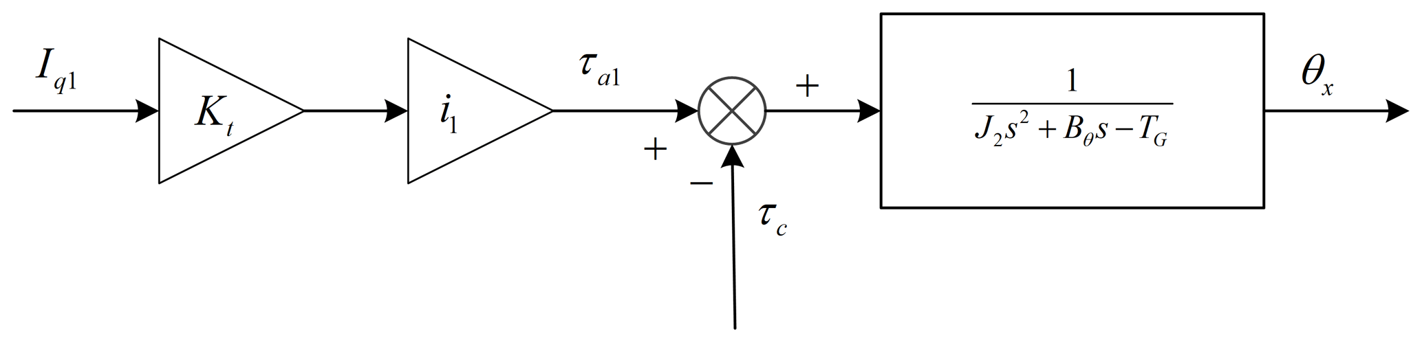
According to Fig. 12, the continuous function can be expressed as:
The zero order holder method is adopted for Z transformation in Eq. (22), and the following equation can be obtained:
In which,
By discretizing Eq. (24), the following equation can be obtained:
In which,
In Eq. (27), τc+ represents positive Coulomb friction and τc− represents negative Coulomb friction.
Set the torque mode through the motor driver, set the specific current size, and drive the haptic interface to rotate. When the motor speed reaches a certain value, take multiple groups of current value Iq1 and rotation angle θx.
For the obtained data, the genetic algorithm in Sect. 3.2 can be used to identify the moment of inertia. The estimated J2 value among search range [0.1–1.1]. The population size was set as 100, and the crossover probability and mutation probability were set as 0.4 and 0.1 respectively. The selection of GA parameters has been carried out by considering the peculiarities of the specific identification problem as well as several preliminary identification tests. In particular, the selected crossover parameter has been defined to give a preference to parental individuals on filial individuals. The selected low variation value is motivated by a limited influence of variation on this specific parameter identification.
The multiple groups of rotation angles calculated by Eq. (26) can be expressed as:
The minimum target value is given as 10−4, and the maximum evolution algebra is 10 000 generations. The evolution of its optimal solution is shown in Fig. 13. The J2 of the recognized moment of inertia is 0.2887 kg m2.
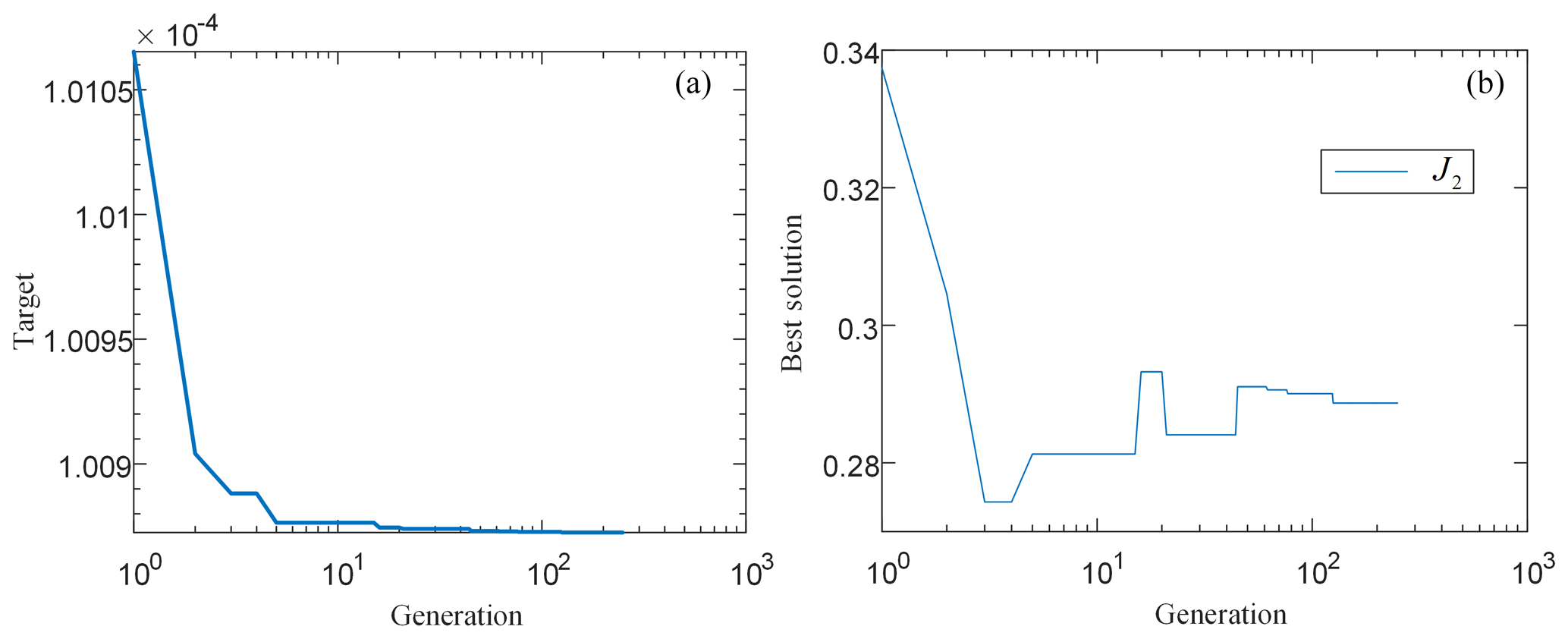
Figure 13Identification process of moment of inertia. (a) The objective function changes with generations; (b) the elite individual changes with generations.
Performming the same operation on the motor 2 as above, and the identified moment of inertia J1+J2 is 0.2989 kg m2. Therefore, J1 is 0.0102 kg m2.
Based on the experimental platform in Fig. 2, the driver is connected to the switch through the X11 terminal, and the switch is connected to the computer. Use Visual Studio C for programming. The computer communicates with the driver via Modbus TCP. Specifically, the program adopts the dynamic mapping function of Modbus. Modbus allows the driver to map any fixed register address to a new register address, and read-write access to the remap parameters by reordering the sequence block. The computer gives instructions to read or change the motor current state by reading or modifying the value in the register.
In this paper, the sampling time of the motor is given as 15 ms, and the quadrature axis current Iq1 and Iq2 size are set as 0. After noise removal, the rotation speed ω1, ω2 and position θm1, θm2 of the two motors at each moment were measured. ω1 and θm1 can be converted to the reducer 1. the reducer 1 output angular speed and position θx are corresponding to them respectively; ω2 and θm2 can be converted to the reducer 2. The reducer 2 output angular speed and position θy are corresponding to them respectively; by substituting ω1 and ω2 into Eq. (14), the friction torque τf1 and τf2 of two degrees of freedom on the haptic interface at the current moment can be obtained. The angular acceleration , of two degrees of freedom of the haptic interface can be calculated by difference method, and they can be expressed as:
In Eq. (29), T is the sampling time of the motor.
At this time, the driver's force on the haptic interface can be obtained through Eq. (13).
In the experiment, the pilot manipulates the haptic interface diagonally and nearly sinusoidal, as shown in Fig. 14a, and records the control force after the kinetic solution. The calculation result of haptic interface force in the whole process is shown in Fig. 14b.
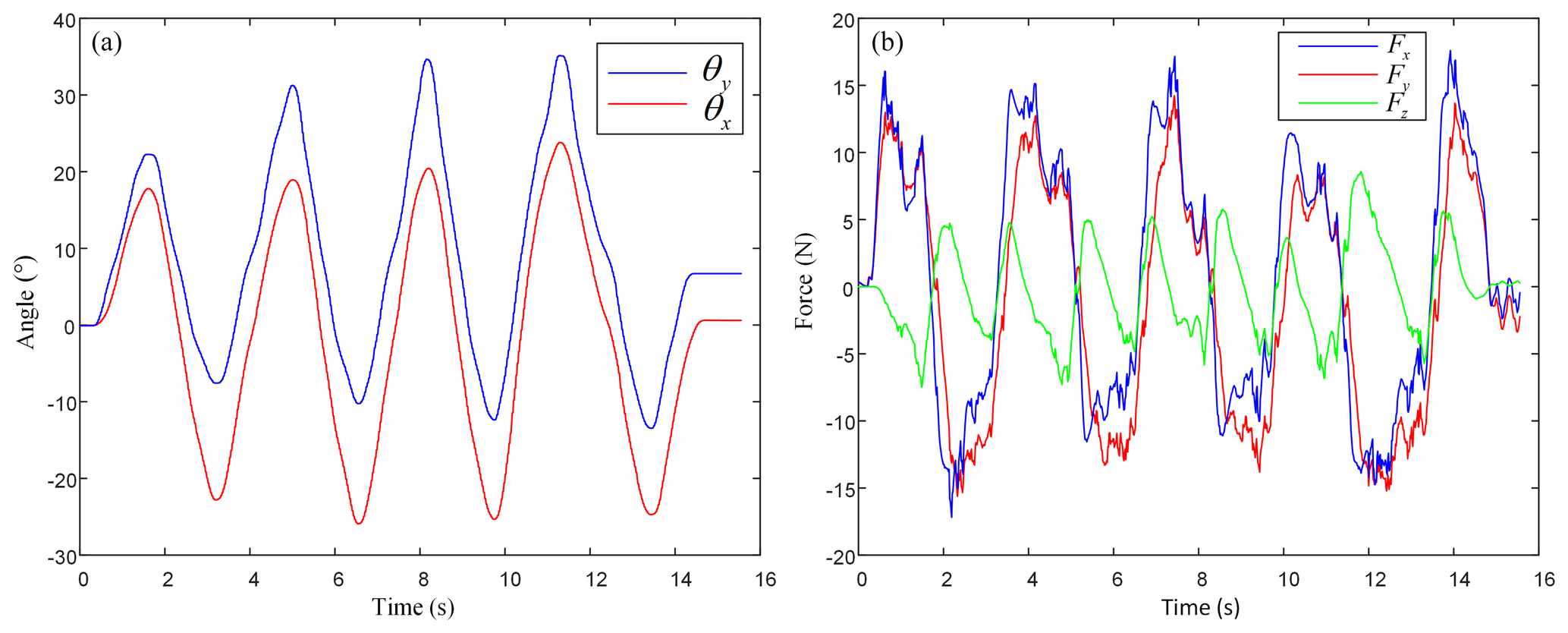
Figure 14Control process of the haptic interface approaching sinusoidal motion. (a) Operating conditions of the haptic interface; (b) calculation results.
Then take the take-off stage and the helicopter hovering to the left for example.
For the control process in the take-off stage, after lifting the total pitch bar, the pilot slowly and uniformly pulls the haptic interface backward. The haptic interface needs to be operated negatively along the x axis to make the helicopter climb steadily, and holds the haptic interface steadily after pulling back to a certain degree. When the helicopter climbs to the target altitude, lay down the haptic interface. The haptic interface needs to be operated forward along the x axis to make the helicopter attitude. The specific control process is shown in Fig. 15. From Fig. 15b, it can be seen that the pilot in t1 moment is pulling the haptic interface in a negative direction towards the x axis and Fx, Fz both are negative. In the t2 stage, the pilot holds the haptic interface for a certain seconds. At this time, because the motor speed is zero, Fx and Fz only equal to gravity. Fx, Fz are all constant positive values. In the t3 stage, the pilot pulls the haptic interface forward along the x axis, therefore, both Fx, Fz are positive. At the t4 stage, the haptic interface returns to its original position, and the values of Fx, Fz back zero. In addition, because the driver did not apply force in the direction of the y axis, Fy was constant zero in the whole process.
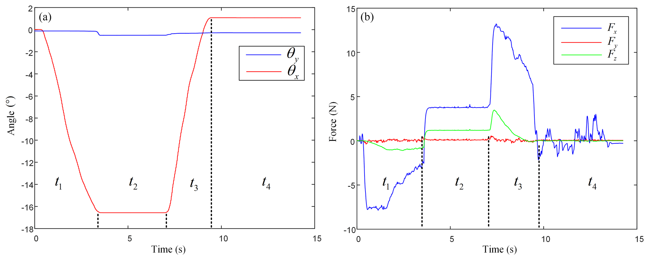
Figure 15Helicopter take-off stage control process. (a) Operating conditions of the haptic interface; (b) calculation results.

Figure 16Helicopter hovering to the left. (a) Operating conditions of the haptic interface; (b) calculation results.
For the control process of helicopter hovering to the left, the pilot slowly and uniformly pulls the haptic interface. The haptic interface needs to be operated forward along the y axis so that the helicopter fuselage tilts to the left. After pulling the haptic interface to a certain extent, the pilot stabilizes the haptic interface. At this time, with the operation of the helicopter pedal, the helicopter can make circular circling. The specific control process is shown in Fig. 16. As can be seen from Fig. 16b, in the t1 stage, the pilot pulls the haptic interface forward along the y axis, which Fy is positive and Fz negative. In the t2 stage, the pilot holds the haptic interface firmly, which Fy is negative value and Fz positive value. Fx was constant zero in the whole process.
It can be seen from the experiments that the control process curve of take-off stage and left hover stage is consistent with the actual driving situation. It can be indicated that proposed identification method for the haptic interface model parameters are feasible and can be applied in the helicopter flight simulator.
In this paper we have addressed the dynamic modelling and parameter identification of a joystick-like haptic interface to be used for helicopter flight simulators. Careful attention has been addressed at the Stribeck friction model and its parameters for an accurate modelling of servomotors. A specific genetic algorithm has been implemented for an accurate identification of the Stribeck friction parameters. A full dynamic model has been developed and implemented as based on Lagrange formulation. Experimental tests show that the proposed identification procedure and haptic interface allow a control of both take-off and left hover stage with results being consistent with the actual helicopter driving. Accordingly, the proposed haptic interface can provide a reliable force feedback even without using expansive force sensors. As future work, we aim at improving the proposed model for a more accurate modelling of friction especially when the velocity is close to zero. Future activities will also include further experimental testing.
All data used in this paper can be obtained on request from the corresponding author.
DZ and JZ wrote the whole paper, HY and TN designed the experiment and dealt with data, GC and SY revised the paper.
The authors declare that they have no conflict of interest.
The authors would like to thank the Hebei Province “Giant Plan” (grant no. 4570031) and the Hebei Province Natural Science Fund (grant no. E2019203431) for supporting this research work.
This research has been supported by the Hebei Province “Giant Plan” (grant no. 4570031) and the Hebei Province Natural Science Fund (grant no. E2019203431).
This paper was edited by Daniel Condurache and reviewed by Adrian Pisla and two anonymous referees.
Azizi, Y. and Yazdizadeh, A.: Passivity-based adaptive control of a 2-DOF serial robot manipulator with temperature dependent joint frictions, Int. J. Adapt. Control, 33, 512–526, https://doi.org/10.1002/acs.2968, 2019.
Balogh, A. and Krstic, M.: Stability of partial difference equations governing control gains in infinite-dimensional backstepping, Syst. Control Lett., 51, 151–164, https://doi.org/10.1016/S0167-6911(03)00222-6, 2004.
Bona, B. and Indri, M.: Friction Compensation in Robotics: an Overview, in: Proceedings of the 44th IEEE Conference on Decision and Control, 15 December 2005, Seville, Spain, 4360–4367, https://doi.org/10.1109/CDC.2005.1582848, 2005.
Broel-Plater, B., Jaroszewski, K., and Dworak, P.: Minimizing the Impact of Non-Linear Stribeck Friction on Positioning of a Servo Drive, in: Proceedings of the 2018 23rd International Conference on Methods & Models in Automation & Robotics (MMAR), 27–30 August 2018, Miedzyzdroje, Poland, 870–875, https://doi.org/10.1109/MMAR.2018.8486112, 2018.
Canudas de Wit, C., Olsson, H., Astrom, K. J., and Lischinsky, P.: A new model for control of systems with friction, IEEE T. Autom. Control, 40, 419–425, https://doi.org/10.1109/9.376053,1995.
Cavallo, A., Natale, C., Pirozzi, S., Visone, C., and Formisano, A.: Feedback Control Systems for Micro-positioning Tasks with Hysteresis Compensation, IEEE T. Magn., 40, 876–879, https://doi.org/10.1109/TMAG.2004.824777, 2004.
Chen, D., Yao, F., and Chai, S.: Sliding Mode Control with Observer for PMSM Based on Stribeck Friction Model, in: Proceedings of the 2016 Chinese Control and Decision Conference, 28–30 May 2016, Hangzhou, Zhejiang, 469–472, https://doi.org/10.1109/CCDC.2016.7531746, 2016.
Ciliza, M. K. and Tomizuka, M.: Friction modelling and compensation for motion control using hybrid neural network models, Eng. Appl. Artif. Intell., 20, 898–911, https://doi.org/10.1016/j.engappai.2006.12.007, 2007.
Fergani, S., Allias, J. F., Briere, Y., and Defay, F.: A novel structure design and control strategy for an aircraft active sidestick, in: Proceedings of the 2016 24th Mediterranean Conference on Control and Automation (MED), 21–24 June 2016, Athens, Greece, 1114–1119, https://doi.org/10.1109/MED.2016.7536014, 2016.
Freidovich, L., Robertsson, A., Shiriaev, A., and Johansson, R.: LuGre-Model-Based Friction Compensation, IEEE T. Contr. Syst. T., 18, 194–200, https://doi.org/10.1109/TCST.2008.2010501, 2010.
Hutton, R. J., Flach, J. M., Brickman, B. J., Hettinger, L. J., Haas, M., and Russell, C. T.: Keeping in touch: kinesthetic-tactile information and fly-by-wire, in: Proceedings of the 38th Annual Meeting of the Human Factors and Ergonomics Society, 24–28 October 1994, Nashville, TN, 26–30, 1994.
Ishikawa, J., Tei, S., Hoshino, D., Izutsu, M., and Kamamichi, N.: Friction compensation based on the LuGre friction model, in: Proceedings of SICE Annual Conference 2010, 18–21 August 2010, Taipei, Taiwan, 2010.
Iwasaki, M., Shibata, T., and Matsui, N.: Disturbance-observer-based nonlinear friction compensation in table drive system, IEEE-ASME T. Mech., 4, 3–8, https://doi.org/10.1109/3516.752078, 1999.
Lichun, B. and Pavelescu, D.: The friction-speed relation and its influence on the critical velocity of stick-slip motion, J. Wear, 82, 277–289, https://doi.org/10.1016/0043-1648(82)90223-x, 1982.
Liu, D.: Genetic Algorithms Based Parameter Identification for Nonlinear Mechanical Servo Systems, in: Proceedings of the 2006 1ST IEEE Conference on Industrial Electronics and Applications, 24–26 May 2006, Singapore, Singapore, 1–5, https://doi.org/10.1109/ICIEA.2006.257322, 2016.
Márton, L. and Lantos, B.: Control of mechanical systems with Stribeck friction and backlash, Syst. Control Lett., 58, 141–147, https://doi.org/10.1016/j.sysconle.2008.10.001, 2009.
Prachyabrued, M. and Robert, O. P.: Development of Attack Helicopter Simulator, in: Proceedings of the 2018 5th Asian Conference on Defense Technology (ACDT), 25–27 October 2018, Hanoi, Vietnam, 31–36, https://doi.org/10.1109/ACDT.2018.8592944, 2018.
Rinaldi, P. and Beckham, K.: Digital Control Loading – a Modular Approach, in: Proceedings of the 1983 American Control Conference, 22–24 June 1983, San Francisco, CA, USA, 269–273, https://doi.org/10.23919/ACC.1983.4788224, 1983.
Wang, H., Sun, Y., and Tian, Y.: Mechanical Structure Design and Robust Adaptive Integral Backstepping Cooperative Control of a New Lower Back Exoskeleton, Stud. Inform. Control, 28, 133–146, https://doi.org/10.24846/v28i2y201902, 2019.
Xu, J., Qiao, M., Wang, W., and Miao, Y.: Fuzzy PID control for AC servo system based on Stribeck friction model, in: Proceedings of the 2011 6th International Forum on Strategic Technology, 22–24 August 2011, Harbin, Heilongjiang, 706–711, https://doi.org/10.1109/IFOST.2011.6021121, 2011.