Use of mixed coordinates in modeling wind turbines including tubular tower

This paper studies the effect of the tower dynamics upon the wind turbine model by using mixed sets of rigid and/or nodal and/or modal coordinates within multibody system dynamics approach. The nodal model exhibits excellent numerical properties, especially in the case where the rotation of the rotor-blade is extremely high, and therefore, the geometric stiffness effect can not be ignored. However, the use of nodal models to describe the flexibility of large multibody systems produces huge size of coordinates and may consume massive computational time in simulation. On the other side, the dynamics of the tower as well as other components of wind turbine remain exhibit small deformations and can be modeled using Cartesian and/or reduced set of modal coordinates. The paper examines a method of using mixed sets of different coordinates in the same model, although there are differences in the scale and the physical interpretation. The equations of motion of the wind-turbine model is presented based on the floating frame of reference formulation. The mixed coordinates vector consists of three sets: Cartesian coordinates set to present the rigid body motion (nacelle and rotor bodies), elastic nodal coordinates for rotating blades, and reduced-order modal coordinates for low speed components and those that deflect by simple motion shapes (circular Tower). Experimental validation has been carried out successfully, and consequently, the proposed model can be utilized for design process, identification and health monitoring aspects.

1 Introduction

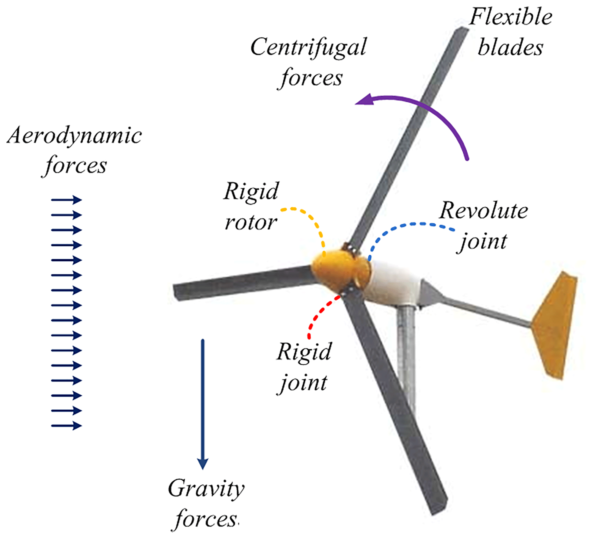
Computational modeling of wind turbines is an important tool in design and control of these dynamic systems. The presence of wind turbines in highly dynamic environment reduces the assumptions that may facilitate the dynamic model, and therefore, the use of multibody system dynamic approach is inevitable. Multibody systems are characterized by two distinguishing features: the system components undergo finite relative rotations, and these components are connected by mechanical joints that impose restrictions on their relative motion (Shabana, 2013). It is therefore can be considered that wind turbines are the real and most important application of flexible multibody dynamics, see Fig. 1. Under the umbrella of the multibody systems, three main approaches can be used to describe the dynamics of a moving body. First, the Newton-Euler formulation that uses a set of Cartesian coordinates to describe the rigid motion of the body and, in addition, the orientational parameters of its local frame that may be assigned at its center of mass, introduced in Shabana (2010). Second, the Floating Frame of Reference (FFR) formulation, which uses a set of Cartesian, orientational and elastic coordinates, in which the deformation of the body with respect to its local frame is described using finite deformations and rotations, more details are presented in Nikravesh and Lin (2005), Nada et al. (2009, 2010) and Wu and Tiso (2014). Finally, the Absolute Nodal Coordinates Formulation (ANCF), that uses a set of global positions and gradients, presented in Gerstmayr (2003), Dibold et al. (2009), Bayoumy et al. (2012a, b) and Nada (2013), to describe the rigid body motion as well as the elastic deformation. The three methods have properties differing in terms of accuracy, complexity and computation efficiency, discussed in Shabana (2008). Naturally, these methods depend strongly on the expected rigid displacement and deformation of the body.

Hansen et al. (2006) have shown a comprehensive review of wind turbine aeroelasticity. Different approaches to structural modeling of wind turbines are addressed in terms of possible instabilities. Nada and Al-Shahrani (2017) have testified that the FFR is best suited for modeling the dynamics of small-size wind turbine, theoretical and experimental validation of using FFR are carried out successfully. Each blade is considered as deformable body (3-D beam element) in the system, the local frame is assigned at the start of the blade. The large reference displacement of the blade is described using a set of absolute Cartesian and orientational parameters (Euler parameters) while the elastic deformation of the blade is described using finite deformations and rotations (elastic coordinates) with respect to the local frame. These elastic coordinates are assumed small, and as a consequence, the stiffness matrix is constant. The mass matrix, on the other hand, is non-linear and exhibits a strong coupling between the reference displacements and the elastic deformations of the body.

It is certainly that the accuracy of the FFR depends on the number of elements used to construct the model. Therefore, a large number of elements must be used and thus huge size of elastic coordinates. Consequently, the use of finite element models to describe flexibility may consume large computational time. Despite the increasing computational capabilities of digital processors, the need remains for using coordinate reduction methods, especially in the case of large multibody systems. A truly straightforward and computationally efficient way of describing deformations is the use of linear deformation modes of the body (Nowakowski et al., 2012; Holzwarth and Eberhard, 2015). These modes can be formulated using a finite element model of the body, and most often, they are eigenmodes of structural vibrations. A set of modal coordinates can describe the elastic deformation of the body instead of using the hug set of elastic nodal coordinates. In this context, Component Mode Synthesis (CMS) is one of the most efficient methods developed to reduce the number of elastic coordinates, in which the model reduction can be achieved by ignoring high deformation modes (Holm-Jørgensen and Nielsen, 2009a, b; Ziegler et al., 2016).

Figure 1 Small-size wind turbine as a multibody system.

Unfortunately, in the case of high-speed rotary machines, such as small-size wind turbines, the use of the reduced-model and the associated modal coordinates face with numerical difficulty (Nada and Al-Shahrani, 2017). In wind turbine application, once the rotor speed reaches the first natural frequency of blade structure, the use of linear form gives wrong solution, and the nonlinear term (geometric stiffness term) should be included in the FFR model. In this case, the elastic coordinates must be utilized in the model construction (Nada et al., 2010).

On the other hand, the tower of the turbine, remains exhibit small deformations and there is no rotations of its local frame; and therefore the modal coordinates can be easily used. The use of modal transformation reduce the number of degrees of freedom and consequently decrease the computational time. But the issue remains how to combine different coordinates in the same model, although there are differences in the scale and the physical interpretation, and their effect on the numerical integration of the mathematical model.

An additional aspect of this study is dealing with the nature of the tower body – most of which are circular shapes – whether solid or hollow. Several publications have presented the finite-element model of rod, which is mostly subjected to high speed rotations and torque applications (Simo and Vu-Quoc, 1991; Weiss, 2002; Koutsovasilis and Beitelschmidt, 2008; Lang et al., 2011). While the application here differs in the exposure of the tower to bending stress more than shear and Euler-Bernoulli beam model can be accurately utilized. Therefore, this paper examines how to calculate the deformation gradient and the resulting strain on the body of the tower in cylindrical coordinates, and then selecting the minimum number of modal coordinates that can be used in the tower model.

This investigation proposes FFR model of wind turbines using three sets of coordinates: Cartesian coordinates plus the Euler parameters to present the rigid body motion (Nacelle and rotor bodies). Elastic nodal coordinates for rotating blades, and modal coordinates for non-rotating bodies (Tower). The paper examines the effectiveness of the proposed FFR formulation in modeling small-size wind turbines as well as the effect of the tower dynamics on the rotor speed.

Figure 2 Beam element of circular cross section within FFR formulation.

2 Dynamics of multibody system

The general dynamic equations of the flexible multibody systems that consist of rigid and flexible can be written as

$$\begin{array}{}\text{(1)}& \left[\begin{array}{cc}\mathbf{M}& {\mathbf{C}}_{\mathit{q}}^{\text{T}}\\ {\mathbf{C}}_{\mathit{q}}& \mathrm{0}\end{array}\right]\left[\begin{array}{c}\ddot{\mathit{q}}\\ \mathit{\lambda }\end{array}\right]=\left[\begin{array}{c}\mathit{Q}\\ {\mathit{Q}}_{\text{d}}\end{array}\right]\end{array}$$

The dynamic coupling between the generalized coordinates, q, is defined using the joint connectivity conditions, C(q)=0, see Sugiyama et al. (2003); Korkealaakso et al. (2009). In Eq. (1), M is the mass matrix, ${\mathbf{C}}_{\mathit{q}}=\frac{\partial \mathbf{C}}{\partial \mathit{q}}$ is the Jacobian of the constraints function, λ is the vector of Lagrange multipliers, and $\ddot{\mathit{q}}$ is the generalized acceleration vector. In the case of using the FFR formulation, the vector

$$\mathit{q}={\left[\begin{array}{cc}{\mathit{q}}_r^{i\text{T}}& {\mathit{q}}_{\text{f}}^{i\text{T}}\end{array}\right]}^{\text{T}}={\left[\begin{array}{ccc}{\mathbf{R}}^{i\text{T}}& {\mathit{\theta }}^{i\text{T}}& {\mathit{q}}_{\text{f}}^{i\text{T}}\end{array}\right]}^{\text{T}}$$

is the generalized coordinates vector. The vector Q, which includes the generalized forces associated with generalized coordinates which is defined as

$$\begin{array}{}\text{(2)}& \mathit{Q}={\mathit{Q}}_{\text{v}}+{\mathit{Q}}_{\text{k}}+{\mathit{Q}}_{\text{e}}\end{array}$$

where Q_v is the vector of centrifugal and Coriolis forces which are quadratic in the velocities, Q_k is the vector of elastic forces, and Q_e is the vector of the external and aerodynamical forces. The vector Q_d absorbs the quadratic velocity terms resulting from the differentiation of the kinematics constraints twice with respect to time, ${\mathit{Q}}_{\text{d}}={\mathbf{C}}_{\mathit{q}}\ddot{\mathit{q}}=-{\left({\mathbf{C}}_{\mathit{q}}\dot{\mathit{q}}\right)}_{\mathit{q}}\dot{\mathit{q}}-\mathrm{2}{\mathbf{C}}_{\mathit{q}t}\dot{\mathit{q}}-{\mathbf{C}}_{tt}$. The reader can review Nada and Al-Shahrani (2017) for full details of each term in Eq. (1).

2.1 FFR Based Nodal Coordinates

In the FFR formulation, element deformation can be described with respect to a frame of reference, this frame is used to describe the large displacements and rotations of body motion. The global position of an arbitrary point P^ij located on the body i within element j, can be written as Shabana (2013):

$$\begin{array}{}\text{(3)}& {\mathit{r}}^{ij}={\mathbf{R}}^i+{\mathbf{A}}^i{\stackrel{\mathrm{‾}}{\mathit{u}}}^{ij}\end{array}$$

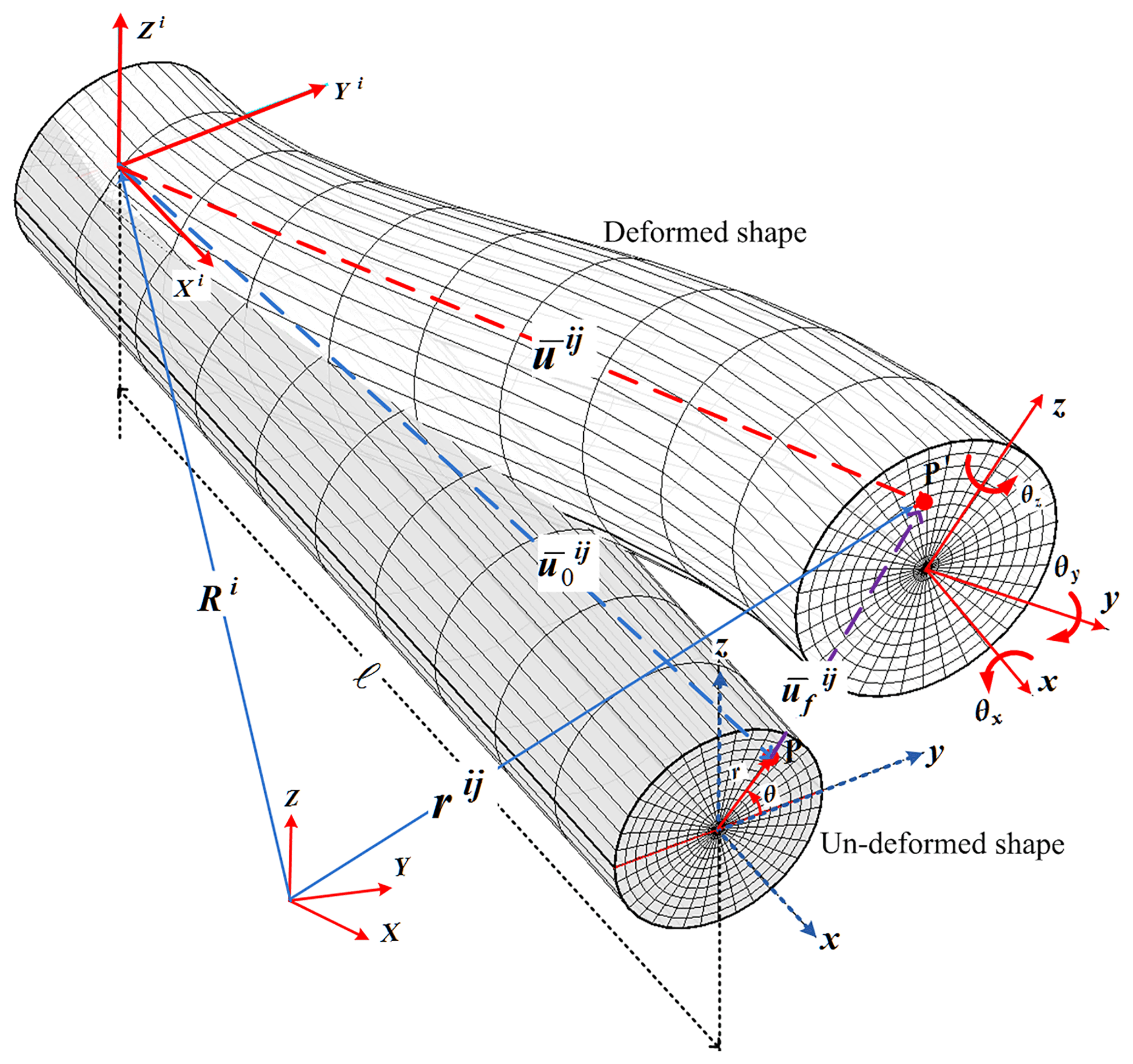
where Rⁱ defines the location of the origin of the body frame xⁱyⁱzⁱ, i.e., floating frame, Aⁱ(θⁱ) is the transformation matrix that defines the orientation of the floating frame xⁱyⁱzⁱ with respect to the inertial frame XYZ as a function of the orientation parameters θⁱ. The vector ${\stackrel{\mathrm{‾}}{\mathit{u}}}^{ij}$ that defines the location of the point P^ij with respect to the floating frame, see Fig. 2, can be expressed in terms of the elastic coordinates as:

$$\begin{array}{}\text{(4)}& {\stackrel{\mathrm{‾}}{\mathit{u}}}^{ij}={\stackrel{\mathrm{‾}}{\mathit{u}}}_{\mathrm{0}}^{ij}+{\stackrel{\mathrm{‾}}{\mathit{u}}}_{\text{f}}^{ij}={\stackrel{\mathrm{‾}}{\mathit{u}}}_{\mathrm{0}}^{ij}+{\mathbf{S}}^{ij}\left({\mathbf{\varkappa }}_{\mathrm{0}}^{ij}\right){\mathit{q}}_{\text{f}}^{ij}\end{array}$$

where ${\stackrel{\mathrm{‾}}{\mathit{u}}}_{\mathrm{0}}^{ij}$ is the position vector of point P in the undeformed configuration. The vector ${\stackrel{\mathrm{‾}}{\mathit{u}}}_{\text{f}}^{ij}$ represents the elastic deformation of the element and defined as ${\stackrel{\mathrm{‾}}{\mathit{u}}}_{\text{f}}^{ij}={\mathbf{S}}^{ij}{\mathit{q}}_{\text{f}}^{ij}$, where ${\mathbf{S}}^{ij}\left({\mathbf{\varkappa }}_{\mathrm{0}}^{ij}\right)$ is the shape function matrix which is space-dependent function along and within the element, however, ${\mathit{q}}_{\text{f}}^{ij}$ is a temporal vector of elastic nodal coordinates of the element j. Thus, if the body is divided into n_e elements, then, the global position vector r^ij can be represented as

$$\begin{array}{}\text{(5)}& {\mathit{r}}^{ij}={\mathbf{R}}^i+{\mathbf{A}}^i{\stackrel{\mathrm{‾}}{\mathit{u}}}_{\mathrm{0}}^{ij}+{\mathbf{A}}^i{\mathbf{S}}^{ij}{\mathbf{B}}_{\mathrm{1}}^{ij}{\mathbf{B}}_{\mathrm{2}}^i{\mathit{q}}_{\text{f}}^i\end{array}$$

where ${\mathbf{B}}_{\mathrm{1}}^{ij}$ is the connectivity matrix and ${\mathbf{B}}_{\mathrm{2}}^i$ is the linear-transformation matrix that imposes the boundary conditions of the element. In this case, ${\mathit{q}}_{\text{f}}^i$ represents the unconstrained vector of nodal coordinates along the body i. Using the matrix ${\mathbf{B}}_{\mathrm{2}}^i$, one can exclude the constrained elastic degrees of freedom from the numerical integration. For example, in the case of rigid connection at particular node, the six elastic degrees of freedom associated with that node can be excluded from the generalized coordinates vector.

Using the displacement field of Eq. (5), one can show that the mass matrix of body i can be assembled as follow

$$\begin{array}{}\text{(6)}& {\mathbf{M}}_{\text{f}}^i=\left[\begin{array}{ccc}{\mathbf{M}}_{\text{RR}}^i& {\mathbf{M}}_{\text{R}\mathit{\theta }}^i& {\mathbf{M}}_{\text{Rf}}^i\\ & {\mathbf{M}}_{\mathit{\theta }\mathit{\theta }}^i& {\mathbf{M}}_{\mathit{\theta }\text{f}}^i\\ \text{sym.}& & {\mathbf{M}}_{\text{ff}}^i\end{array}\right]\end{array}$$

where ${\mathbf{M}}_{\text{RR}}^i$ matrix represents the mass matrix associated with the translational coordinates of the body reference. The matrix ${\mathbf{M}}_{\text{R}\mathit{\theta }}^i$ represents the inertia coupling between the rigid body translation and the rigid body rotation. The matrix ${\mathbf{M}}_{\mathit{\theta }\mathit{\theta }}^i$ is associated with the rotational coordinates of the body reference. The submatrices ${\mathbf{M}}_{\text{Rf}}^i$ and ${\mathbf{M}}_{\mathit{\theta }\text{f}}^i$ represent the coupling between the reference motion and elastic deformation. The matrix ${\mathbf{M}}_{\text{ff}}^i$ is the summation elementary mass matrices ${\mathbf{M}}_{\text{ff}}^{ij}$. For n_e finite elements and can be written as:

$$\begin{array}{}\text{(7)}& {\mathbf{M}}_{\text{ff}}^i={\mathbf{B}}_{\mathrm{2}}^{i\text{T}}\left[\underset{j=\mathrm{1}}{\sum ^{n_e}}{\mathbf{B}}_{\mathrm{1}}^{ijT}{\mathbf{M}}_{\text{ff}}^{ij}{\mathbf{B}}_{\mathrm{1}}^{ij}\right]{\mathbf{B}}_{\mathrm{2}}^i\end{array}$$

where ${\mathbf{M}}_{\text{ff}}^{ij}={\int }_{V^{ij}}{\mathit{\rho }}^i{\left[{\mathbf{S}}^{ij}\right]}^{\text{T}}\left[{\mathbf{S}}^{ij}\right]\text{d}{V}^{ij}$ is the mass matrix of element j. Similarly, the assembled stiffness matrix can be written as:

$$\begin{array}{}\text{(8)}& {\mathbf{K}}_{\text{ff}}^i={\mathbf{B}}_{\mathrm{2}}^{i\text{T}}\left[\sum _{j=\mathrm{1}}^{n_e}{\mathbf{B}}_{\mathrm{1}}^{ijT}{\mathbf{K}}_{\text{ff}}^{ij}{\mathbf{B}}_{\mathrm{1}}^{ij}\right]{\mathbf{B}}_{\mathrm{2}}^i\end{array}$$

The stiffness matrix of the element ${\mathbf{K}}_{\text{ff}}^{ij}$ is constant matrix that appear in the linear structural systems and can be found in Shabana (2013). In the FFR formulation, which is linear in the local frame of reference, high order terms related to the deformation of a beam element are ignored. That is why in the case of high rotational speeds or large deformations, some axial and bending effects need to be taken into consideration in addition to the linear beam model. This is called the geometric stiffening, which is most important effect that is neglected in the linear FFR formulation. In wind turbine application, large rigid body motion are taken into account while, however, large deformations can be neglected.

2.2 3-D Beam Element with Circular Cross Section

For the two-nodes 3D-beam element used in this investigation, the nodal coordinates ${\mathit{q}}_{\text{f}}^{ij}$ of body i, element j is given by:

$$\begin{array}{cccccc}\underset{\mathrm{12}\times \mathrm{1}}{{\mathit{q}}_{\text{f}}^{ij}}=\mathit{\{}{u}_{\mathrm{0}}^{j,\mathrm{1}}& v_{\mathrm{0}}^{j,\mathrm{1}}& w_{\mathrm{0}}^{j,\mathrm{1}}& \mathrm{\cdots }& & \\ & {\mathit{\theta }}_x^{j,\mathrm{1}}& {\mathit{\theta }}_y^{j,\mathrm{1}}& {\mathit{\theta }}_z^{j,\mathrm{1}}& \mathrm{\cdots }& \\ & & u_{\mathrm{0}}^{j,\mathrm{2}}& v_{\mathrm{0}}^{j,\mathrm{2}}& w_{\mathrm{0}}^{j,\mathrm{2}}& \mathrm{\cdots }\\ & & & {\mathit{\theta }}_x^{j,\mathrm{2}}& {\mathit{\theta }}_y^{j,\mathrm{2}}& {\mathit{\theta }}_z^{j,\mathrm{2}}{\mathit{\}}}^{\text{T}}\end{array}$$

The subscript 0, refers to the centroidal axis, the complete set of nodal coordinates can be assembled as

$$\begin{array}{}\text{(10)}& \underset{n_{\text{f}}\times \mathrm{1}}{{\mathit{q}}_{\text{f}}^i}={\left[\begin{array}{cccc}{\mathit{q}}_{\text{f}}^{i,\mathrm{1}T}& {\mathit{q}}_{\text{f}}^{i,\mathrm{2}T}& \mathrm{\cdots }& {\mathit{q}}_{\text{f}}^{i,\left(n_e+\mathrm{1}\right)T}\end{array}\right]}^{\text{T}}\end{array}$$

such that ${\mathit{q}}_{\text{f}}^{ij}={\mathbf{B}}_{\mathrm{1}}^{ij}{\mathbf{B}}_{\mathrm{2}}^i{\mathit{q}}_{\text{f}}^i$, the dimension of the ${\mathit{q}}_{\text{f}}^i$ vector is n_f×1, where $n_{\text{f}}=\left(n_e+\mathrm{1}\right)\times \mathrm{6}$ are the total number of elastic degrees of freedom of the flexible body. The 3-D beam element of rectangular cross section is used in modeling wind turbine blades in Nada and Al-Shahrani (2017). However, when the tower is included into the turbine model, the beam element with circular cross section should be used instead. In this case, the coordinates of the material point in the undeformed configuration with respect to the floating frame are described interms of $\left(x,r,\mathit{\theta }\right)$. Thus, the shape function, which defined for beams of rectangular cross section should be mapped into cylindrical coordinates so that the elements match the circular geometry of the cross section.

The Cartesian coordinates are related to the cylindrical coordinates, see Fig. 2, by

$$\begin{array}{}\text{(11)}& \left.\begin{array}{l}x=x\\ y=r\cos \left(\mathit{\theta }\right)\\ z=r\sin \left(\mathit{\theta }\right)\end{array}\right\}\end{array}$$

Thus, the deformation gradient described in cylindrical coordinates $\mathit{\varrho }:\left(x,r,\mathit{\theta }\right)$ can be written as Huang et al. (2013):

$$\begin{array}{}\text{(12)}& \mathbf{D}={\displaystyle \frac{\partial {\stackrel{\mathrm{‾}}{\mathit{u}}}_{fp}}{\partial \mathit{\varrho }}}=\left[\begin{array}{ccc}\frac{\partial u}{\partial x}& \frac{\partial u}{\partial r}& \frac{\partial u}{\partial \mathit{\theta }}\\ \frac{\partial \mathit{\varrho }}{\partial x}& \frac{\partial \mathit{\varrho }}{\partial r}& \frac{\partial \mathit{\varrho }}{\partial \mathit{\theta }}\\ \frac{\partial \mathit{\vartheta }}{\partial x}& \frac{\partial \mathit{\vartheta }}{\partial r}& \frac{\partial \mathit{\vartheta }}{\partial \mathit{\theta }}\end{array}\right]\end{array}$$

Based on the deformation gradient in Eq. (12), one can conclude that the terms of shearing strains of beam element with circular cross area can be formulated as

$$\begin{array}{ll}{\displaystyle }& {\displaystyle }{\mathit{ϵ}}_{xy}=\cos \mathit{\theta }\left({\mathbf{D}}_{(\mathrm{1},\mathrm{2})}+{\mathbf{D}}_{(\mathrm{2},\mathrm{1})}\right)-\sin \mathit{\theta }\left({\displaystyle \frac{{\mathbf{D}}_{(\mathrm{1},\mathrm{3})}}{r}}+{\mathbf{D}}_{(\mathrm{3},\mathrm{1})}\right)\\ {\displaystyle }& {\displaystyle }{\mathit{ϵ}}_{xz}=\cos \mathit{\theta }\left({\mathbf{D}}_{(\mathrm{3},\mathrm{1})}+{\displaystyle \frac{{\mathbf{D}}_{(\mathrm{1},\mathrm{3})}}{r}}\right)-\sin \mathit{\theta }\left({\mathbf{D}}_{(\mathrm{1},\mathrm{2})}+{\mathbf{D}}_{(\mathrm{2},\mathrm{1})}\right)\end{array}$$

The axial component ϵ_xx remains the same as for rectangular cross section, presented in Nada and Al-Shahrani (2017). In order to match the cylindrical coordinates of the 3-D beam with circular cross section, the non-dimensional parameters $\mathit{\xi },\mathit{\eta },\mathit{\zeta }$ of the shape function should be altered to

$$\begin{array}{}\text{(13)}& \mathit{\xi }={\displaystyle \frac{x}{\mathrm{\ell }}},\mathit{\eta }={\displaystyle \frac{r\cos \mathit{\theta }}{\mathrm{\ell }}},\mathit{\zeta }={\displaystyle \frac{r\sin \mathit{\theta }}{\mathrm{\ell }}}.\end{array}$$

The variables of volume integration are the parameters $\left(x,r,\mathit{\theta }\right)$ and volume integration boundaries are altered to $V^{ij}=\underset{\mathrm{0}}{\overset{\mathrm{\ell }}{\int }}\mathrm{\cdots }\underset{-\mathit{\pi }}{\overset{+\mathit{\pi }}{\int }}\mathrm{\cdots }\underset{\mathrm{0}}{\overset{R}{\int }}\mathrm{\cdots }r\text{d}r\text{d}\mathit{\theta }\text{d}x$. Using the mapped forms described above, the dynamic terms can be updated for circular cross section 3-D beams.

Figure 3 Interconnected bodies of wind turbine.

2.3 FFR Based Modal Coordinates

Using the modal analysis techniques; a reduced set of eigenvectors of the free vibration discrete equations of motion as flexible modal coordinates. The reduction is achieved by eliminating the high frequency modes, which carry little energy. Modal reduction offers an efficient way to reduce the number of elastic degrees of freedom, i.e, n_f, with the minimum deterioration in accuracy. The vector ${\mathit{q}}_{\text{f}}^i$ can be written in terms of the reduced vector of modal coordinates ${\mathit{p}}_{\text{f}}^i$ as:

$$\begin{array}{}\text{(14)}& \underset{n_{\text{f}}\times \mathrm{1}}{{\mathit{q}}_{\text{f}}^i}=\underset{n_{\text{f}}\times n_{\text{m}}}{{\mathbf{B}}_{\text{mf}}^i}\underset{n_{\text{m}}\times \mathrm{1}}{{\mathit{p}}_{\text{f}}^i}\end{array}$$

where B_mf is a non-square modal transformation matrix, whose columns define the modes of deformation, where n_f is the number of elastic degrees of freedom, n_m is the number of modal coordinates. Using the preceding equations, a significant reduction in the problem dimensionality can be achieved. In this case, the following transformation must be carried out:

$$\begin{array}{}\text{(15)}& \left.\begin{array}{l}{\mathbf{M}}_{\text{pp}}^i={\mathbf{B}}_{\text{mf}}^{i\text{T}}{\mathbf{M}}_{\text{ff}}^i{\mathbf{B}}_{\text{mf}}^i\\ {\mathbf{M}}_{\text{Rp}}^i={\mathbf{M}}_{\text{Rf}}^i{\mathbf{B}}_{\text{mf}}^i\\ {\mathbf{M}}_{\mathit{\theta }\text{p}}^i={\mathbf{M}}_{\mathit{\theta }\text{f}}^i{\mathbf{B}}_{\text{mf}}^i\end{array}\right\}\end{array}$$

also,

$$\begin{array}{}\text{(16)}& \left.\begin{array}{l}{\mathbf{K}}_{\text{pp}}^i={\mathbf{B}}_{\text{mf}}^{i\text{T}}{\mathbf{K}}_{\text{ff}}^i{\mathbf{B}}_{\text{mf}}^i\\ {\mathit{Q}}_{\text{v}}^p={\mathbf{B}}_{\text{mf}}^{i\text{T}}{\mathit{Q}}_{\text{v}}^f\\ {\mathit{Q}}_{\text{ex}}^p={\mathbf{B}}_{\text{mf}}^{i\text{T}}{\mathit{Q}}_{\text{ex}}^f\end{array}\right\}\end{array}$$

The constraint Jacobian matrix with respect to the new set of coordinates can be expressed by using the following relation:

$$\begin{array}{}\text{(17)}& {\mathbf{C}}_{\mathit{p}}^i={\displaystyle \frac{\partial {\mathbf{C}}^i}{\partial {\mathit{p}}^i}}={\mathbf{C}}_{\mathit{q}}^i{\mathbf{B}}_{\text{m}}^i\end{array}$$

where ${\mathit{p}}^i={\left[\begin{array}{cc}{\mathit{q}}_r^{i\text{T}}& {\mathit{p}}_{\text{f}}^{i\text{T}}\end{array}\right]}^{\text{T}}={\left[\begin{array}{ccc}{\mathbf{R}}^{i\text{T}}& {\mathit{\theta }}^{i\text{T}}& {\mathit{p}}_{\text{f}}^{i\text{T}}\end{array}\right]}^{\text{T}}$ is the reduced generalized coordinates vector interms of the modal coordinates ${\mathit{p}}_{\text{f}}^i$, The transformation matrix ${\mathbf{B}}_{\text{m}}^i$ can be written as:

$$\begin{array}{}\text{(18)}& {\mathbf{B}}_{\text{m}}^i=\left[\begin{array}{cc}\mathbf{I}& \mathbf{0}\\ \mathbf{0}& {\mathbf{B}}_{\text{mf}}^i\end{array}\right]\end{array}$$

The modal transformation matrix ${\mathbf{B}}_{\text{mf}}^i$ can be normalized with respect to the mass matrix or with respect to the stiffness matrix (Nada et al., 2010). In this paper, the modal transformation is normalized with respect to the mass matrix such that:

$$\begin{array}{}\text{(19)}& \left.\begin{array}{l}\underset{n_{\text{m}}\times n_{\text{m}}}{{\mathbf{M}}_{\text{pp}}^i}=\mathbf{I}\\ \underset{n_{\text{m}}\times n_{\text{m}}}{{\mathbf{K}}_{\text{pp}}^i}=\left[\begin{array}{cccc}{\mathit{\omega }}_{\mathrm{1}}^{\mathrm{2}}& \mathrm{0}& \mathrm{\cdots }& \mathrm{0}\\ \mathrm{0}& {\mathit{\omega }}_{\mathrm{2}}^{\mathrm{2}}& & \mathrm{0}\\ \mathrm{⋮}& & \mathrm{\ddots }& \mathrm{⋮}\\ \mathrm{0}& \mathrm{0}& & {\mathit{\omega }}_{n_{\text{m}}}^{\mathrm{2}}\end{array}\right]\end{array}\right\}\end{array}$$

By using the coordinates reduction, the equations of motion, Eq. (1) can be modified into the following form

$$\begin{array}{}\text{(20)}& \left[\begin{array}{cc}{\mathbf{M}}_{\mathit{p}}& {\mathbf{C}}_{{\mathit{p}}^{\text{T}}}\\ \mathbf{C}{}_{\mathit{p}}& \mathrm{0}\end{array}\right]\left[\begin{array}{c}\ddot{\mathbf{p}}\\ \mathit{\lambda }\end{array}\right]=\left[\begin{array}{c}{\mathit{Q}}_{\text{v}}^p+{\mathit{Q}}_{\text{k}}^p+{\mathit{Q}}_e^p\\ {\mathit{Q}}_{\text{d}}^p\end{array}\right]\end{array}$$

The next section presents the multibody model of wind turbine with tower dynamics. Once the modal transformation matrix of the tower is obtained, the body model can be integrated to the rotor-blade system constructed in Nada and Al-Shahrani (2017). The Nacelle is rigidly attached at the top of the tower, which can be approximated as 3-D beam with circular cross section, and the kinematic constraints function is expressed as shown in Korkealaakso et al. (2009).

3 Multibody mixed coordinates model

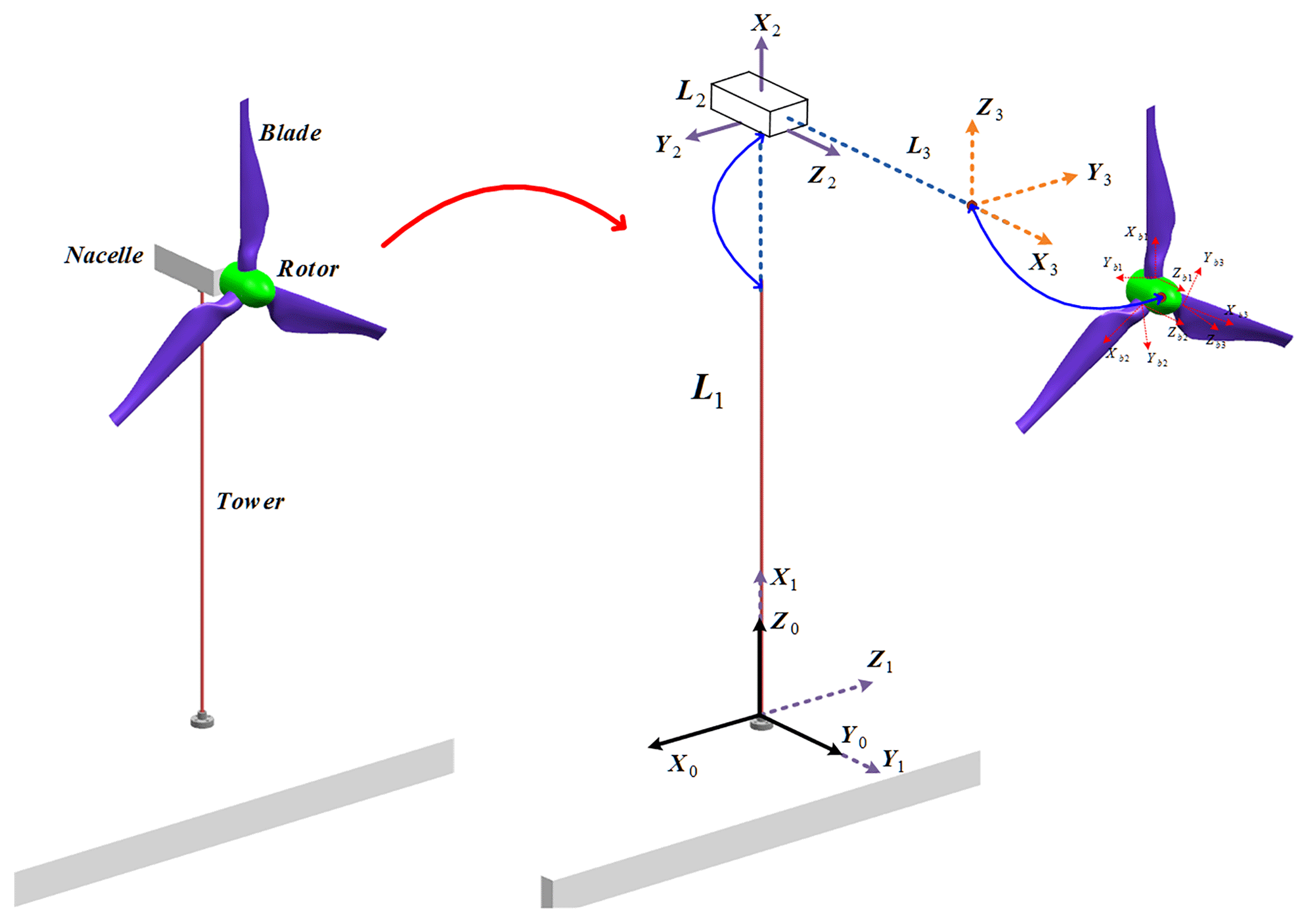
The complete model of wind turbine consist of flexible tower (1), rigid nacelle (2), rigid rotor (3), and a number of flexible blades (b₁→b_n), see Fig. 3. The flexibility of the tower (with circular cross section) can be considered small, and therefore, linear terms of strain can be utilized, and consequently, modal coordinates is recommended for implementation. The nacelle and the rotor can be considered rigid enough such that the selected modes are nil, i.e., ${\mathit{p}}_{\text{f}}^i=\left[\right],$ $i=\mathrm{2},\mathrm{3}$. The nacelle can be considered as 3-D beam with rectangular cross section while the rotor can be considered as 3-D beam with circular cross section. The rotating blades can be modeled as a number of 3-D beams utilizing the corresponding number of elastic coordinates. It should be mentioned that, the term of geometric stiffness is included into the blade's models to avoid wrong simulation results, if the rotational speed is approached from the first natural frequency of the blade (Nada and Al-Shahrani, 2017). The use of nodal models facilitates mathematical integration and helps solve numerical stiffness problems results from modal transformation. Therefore, the elastic nodal coordinates are used for describing the dynamics of the rotating blades. Thus, the generalized coordinates vector, in this case, consists of a mixed set of coordinates, i.e.,

$$\mathit{\psi }={\left[\begin{array}{cccccc}\underset{\left(\mathrm{7}+n_{\text{m}}\right)\times \mathrm{1}}{{\mathit{p}}^{\left(\mathrm{1}\right)T}}& \underset{\left(\mathrm{7}\right)\times \mathrm{1}}{{\mathit{q}}_{\text{r}}^{\left(\mathrm{2}\right)T}}& \underset{\left(\mathrm{7}\right)\times \mathrm{1}}{{\mathit{q}}_{\text{r}}^{\left(\mathrm{3}\right)T}}& \underset{\left(\mathrm{7}+n_{\text{f}}\right)\times \mathrm{1}}{{\mathit{q}}^{\left(b_{\mathrm{1}}\right)T}}& \mathrm{\cdots }& \underset{\left(\mathrm{7}+n_{\text{f}}\right)\times \mathrm{1}}{{\mathit{q}}^{\left(b_n\right)T}}\end{array}\right]}^{\text{T}},$$

such that ${\mathit{p}}^i={\left[\begin{array}{ccc}{\mathbf{R}}^{i\text{T}}& {\mathit{\theta }}^{i\text{T}}& {\mathit{p}}_{\text{f}}^{i\text{T}}\end{array}\right]}^{\text{T}}$, ${\mathit{q}}_{\text{r}}^i={\left[\begin{array}{cc}{\mathbf{R}}^{i\text{T}}& {\mathit{\theta }}^{i\text{T}}\end{array}\right]}^{\text{T}}$, and ${\mathit{q}}^i={\left[\begin{array}{ccc}{\mathbf{R}}^{i\text{T}}& {\mathit{\theta }}^{i\text{T}}& {\mathit{q}}_{\text{f}}^{i\text{T}}\end{array}\right]}^{\text{T}}$, where θ is the Euler parameters of the body, p_f is the modal coordinates, and q_f is the elastic nodal coordinates. Note that n_m is the number of selected modes, n_f is the number of elastic coordinates for each blade, and b_n is the number of rotating blades.

Figure 4 Frequency response function of the tower.

As shown in Fig. 3, the tower is fixed to the ground via rigid joint, the body frame is transformed from the global frame such that the x-axis orients to the axial direction. The free end of the tower is connected to the nacelle through rigid joint, which is connected in the rotor via revolute joint. In the case of three rotating blades, other three rigid joints are implemented to connect these blades with the rotor body. These joints introduce the constraints function C(ψ) that relates the relative motion between the interconnected bodies. The Jacobian of the constraints ${\mathbf{C}}_{\mathit{\psi }}=\frac{\partial \mathbf{C}\left(\mathit{\psi }\right)}{\partial \mathit{\psi }}$ can be assemblies diagonally, and the force vectors can be staked vertically for each body respectively. The equations of motion of the complete small-size wind turbine model can be assembled as expressed in Eq. (21), where $n_{\text{rm}}=\mathrm{7}+n_{\text{m}}$, $n_{\text{rf}}=\mathrm{7}+n_{\text{f}}$.

Equation (21) can be solved for the mixed generalized coordinates vector $\ddot{\mathit{\psi }}$ as well as the vector of Lagrange multipliers λ. The direct integration of $\ddot{\mathit{\psi }}$ can be carried out given proper initial conditions. The gyroscopic motion of the rotor, i.e., body (3), can be examined by estimating the rotation about the local axis Y₃ and/or Z₃. The angular velocities ${\stackrel{\mathrm{‾}}{\mathit{\omega }}}^{\left(\mathrm{3}\right)}$ with respect to the local frame (XYZ)₃ can be obtained using the time rate of Euler parameters as ${\stackrel{\mathrm{‾}}{\mathit{\omega }}}^{\left(\mathrm{3}\right)}={\stackrel{\mathrm{‾}}{\mathbf{G}}}^{\left(\mathrm{3}\right)}$ ${\dot{\mathit{\theta }}}^{\left(\mathrm{3}\right)}$, where ${\stackrel{\mathrm{‾}}{\mathbf{G}}}^{\left(\mathrm{3}\right)}$ is the transformation matrix depends on θ⁽³⁾ (Shabana, 2013). Furthermore, the equations of motion can be used to examine the sensitivity of rotor speed against slight gyroscopic torques. The generalized forces can be then estimated as ${\mathit{Q}}_{\mathit{\theta }}^{\left(\mathrm{3}\right)}={\stackrel{\mathrm{‾}}{\mathbf{G}}}^{\left(\mathrm{3}\right)T}{\stackrel{\mathrm{‾}}{\mathit{T}}}^{\left(\mathrm{3}\right)}$, where ${\stackrel{\mathrm{‾}}{\mathit{T}}}^{\left(\mathrm{3}\right)}$ is the torque vector defined in the rotor's frame.

Table 1 Eigen-Frequencies of tower body.

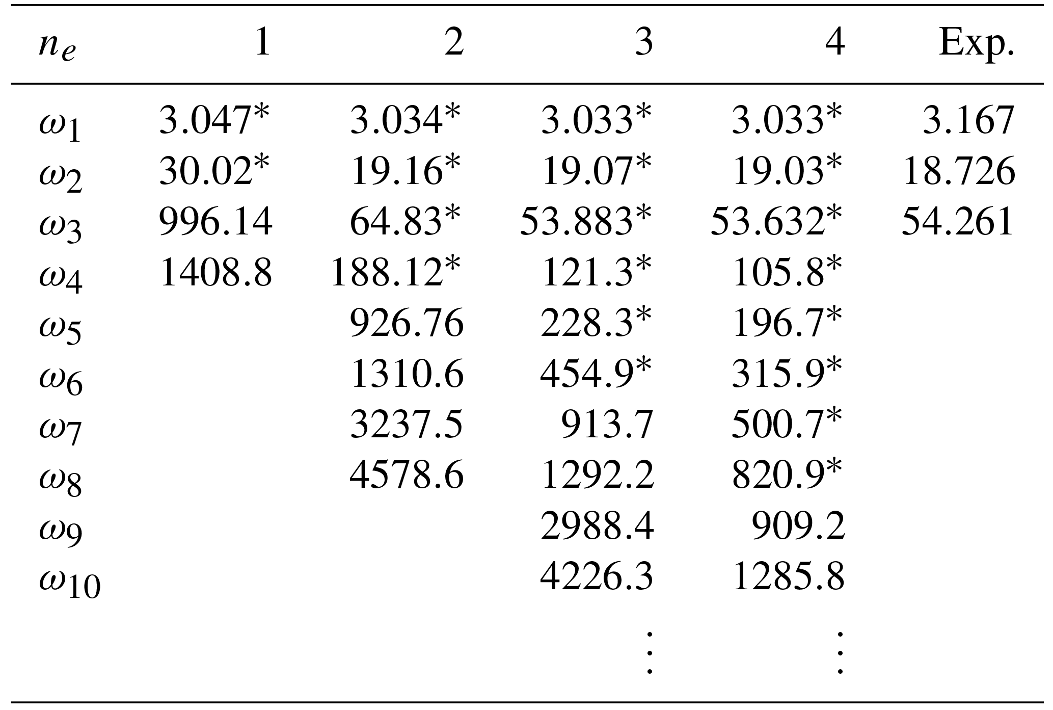
^* Duplication of some frequencies.

Figure 5 First three modes of tower in Y−Z plan.

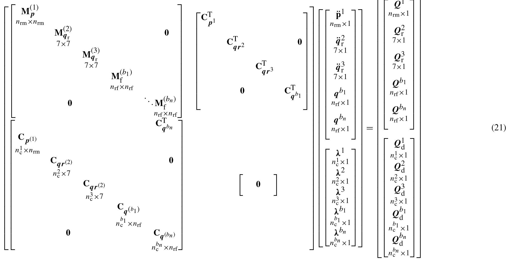
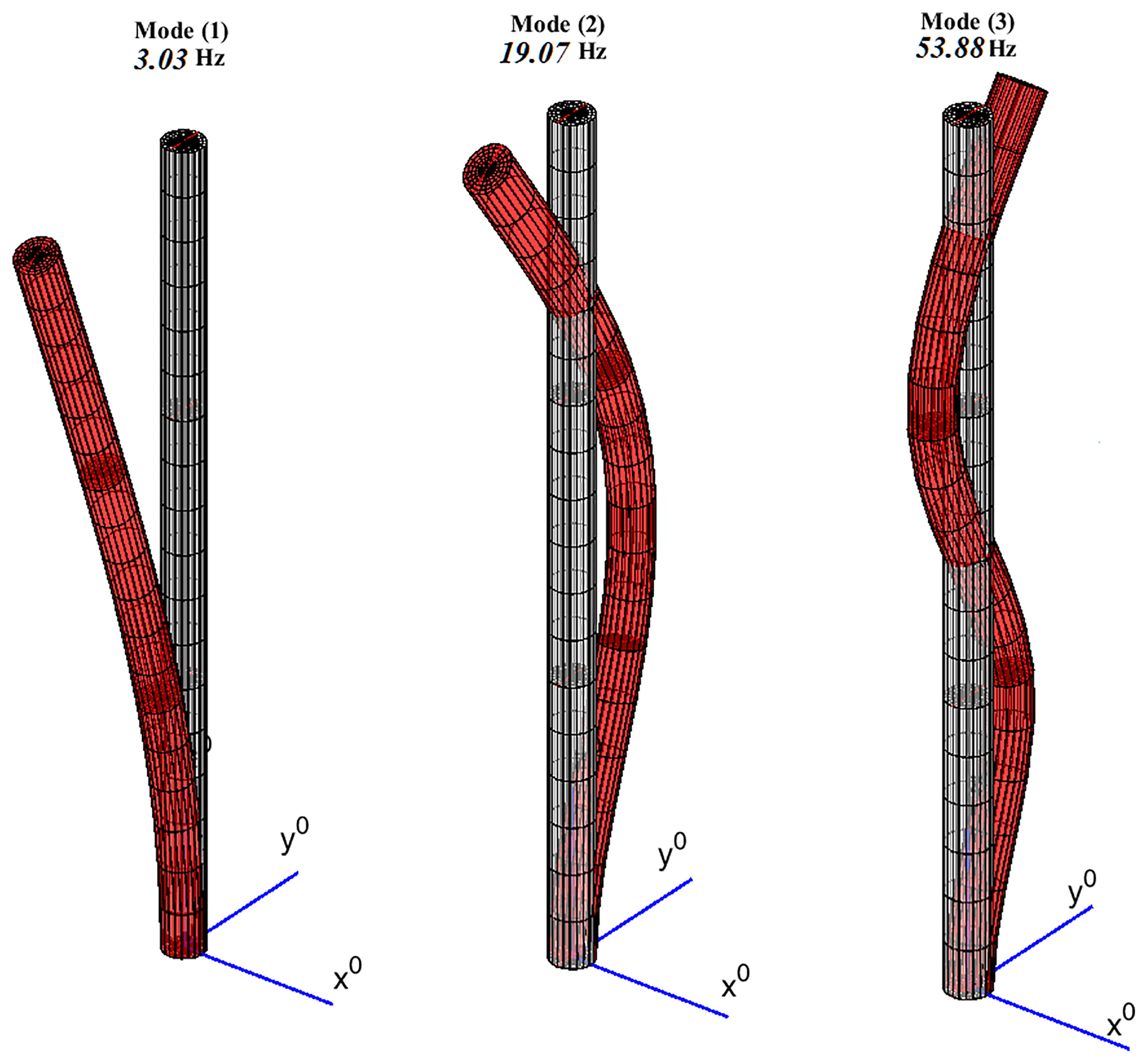
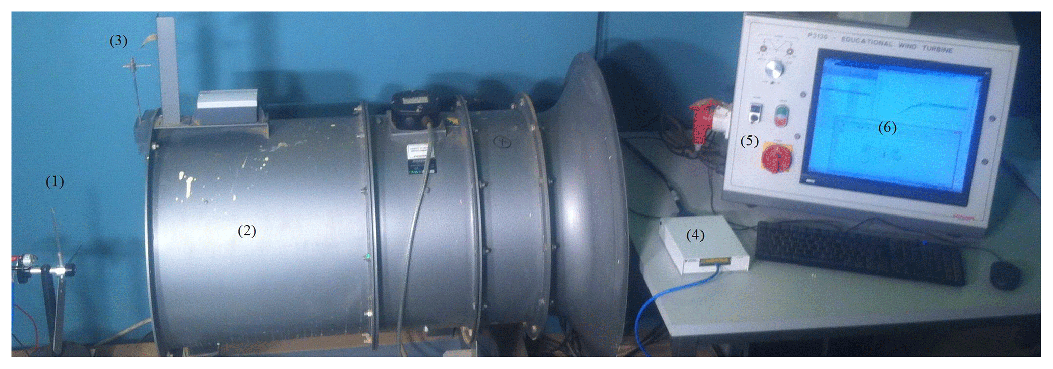
Figure 6 Test-rig: (1) wind turbine, (2) wind generator, (3) Pitot tube, (4) Data acquisition, (5) wind speed controller, (6) datalogging display.

Figure 7 Transverse displacement of the Nacelle at β=25^∘.

4 Numerical and experimental study

The wind turbine prototype is constructed using copper rod of 6 mm diameter, as a flexible tower of 500 mm long. The rotor diameter is 300 mm, i.e., the blade length is 150 mm long, with 27 mm width and 2 mm thickness. Three blades of aluminum are utilized in the prototype of this study. In order to select the proper number of modes, the frequency identification test, based on the Frequency Response Function (FRF), has been carried out. The obtained results are compared with the estimated frequencies based on the mass and stiffness matrices of circular 3-D beam element. As shown in Fig. 4 and Table 1, it can be concluded that the selection of three elements for modeling the tower is sufficient to obtain results that are close to the experimental values. Thus, tower is modeled using three beam elements of circular cross section. Note that the first node is constrained, i.e., fixed-free boundary condition, and therefore $n_{\text{f}}^{\left(\mathrm{1}\right)}=\mathrm{18}$. The lowest natural frequencies of the tower are 3.03, 19.07 and 53.88 Hz, the first three mode shapes are shown in Fig. 5. In Table 1, the asterisk indicates the duplication of some frequencies. This is due to the similarity nature of the beam geometry in (y−z) and (x−z) plans. Consequently, the mode shape matrix ${\mathbf{B}}_{\text{mf}}^{\left(\mathrm{1}\right)}$ of the tower can be estimated to reflect only the transverse motion in the (Y₀−Z₀) plan, see Table 1.

The wind turbine prototype is fixed in the front of the wind generator as shown in Fig. 6, and connected to tachogenerator to measure the output angular velocity. Data Acquisition NI PCI-6259 (16-Bit, 1 MS s⁻¹) is used for collecting the measured data. High sensitivity multi-axis accelerometer is attached with the Nacelle, to measure the induced acceleration, which can be integrated twice to obtain the displacement, see Yin et al. (2012).

$$\begin{array}{}\text{(22)}& \underset{\mathrm{18}\times \mathrm{3}}{{\mathbf{B}}_{\text{mf}}^{\left(\mathrm{1}\right)}}=\left[\begin{array}{ccc}\mathrm{0}& \mathrm{0}& \mathrm{0}\\ -\mathrm{0.6557}& \mathrm{2.3582}& \mathrm{2.968}\\ -\mathrm{0.0542}& \mathrm{0.0182}& -\mathrm{0.1167}\\ \mathrm{0}& \mathrm{0}& \mathrm{0}\\ \mathrm{0.2961}& -\mathrm{0.0546}& -\mathrm{0.2606}\\ -\mathrm{3.5826}& \mathrm{7.0506}& -\mathrm{6.6290}\\ \mathrm{0}& \mathrm{0}& \mathrm{0}\\ -\mathrm{2.1663}& \mathrm{1.6930}& -\mathrm{2.6173}\\ -\mathrm{0.1790}& \mathrm{0.0131}& \mathrm{0.1029}\\ \mathrm{0}& \mathrm{0}& \mathrm{0}\\ \mathrm{0.4285}& \mathrm{0.0916}& -\mathrm{0.1990}\\ -\mathrm{5.1845}& -\mathrm{11.83}& -\mathrm{5.0624}\\ \mathrm{0}& \mathrm{0}& \mathrm{0}\\ -\mathrm{3.9608}& -\mathrm{3.997}& \mathrm{3.9891}\\ -\mathrm{0.3274}& -\mathrm{0.0309}& -\mathrm{0.1568}\\ \mathrm{0}& \mathrm{0}& \mathrm{0}\\ \mathrm{0.4506}& \mathrm{0.148}& \mathrm{1.2467}\\ -\mathrm{5.4521}& -\mathrm{19.129}& \mathrm{31.7107}\end{array}\right]\end{array}$$

Figure 8 Comparison of rotor velocity at β=25^∘.

Figure 9 Comparison of rotor velocity at β=15^∘.

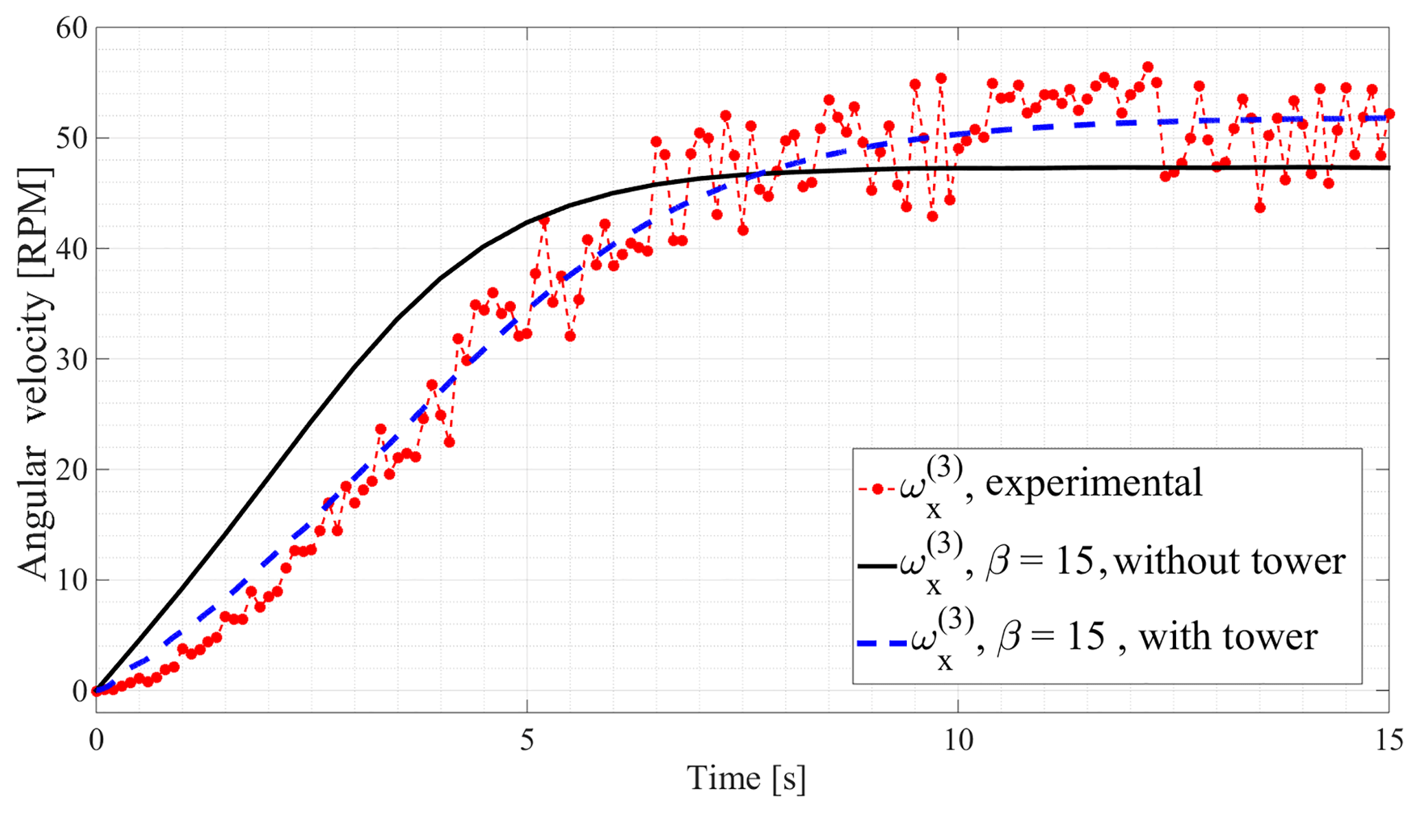
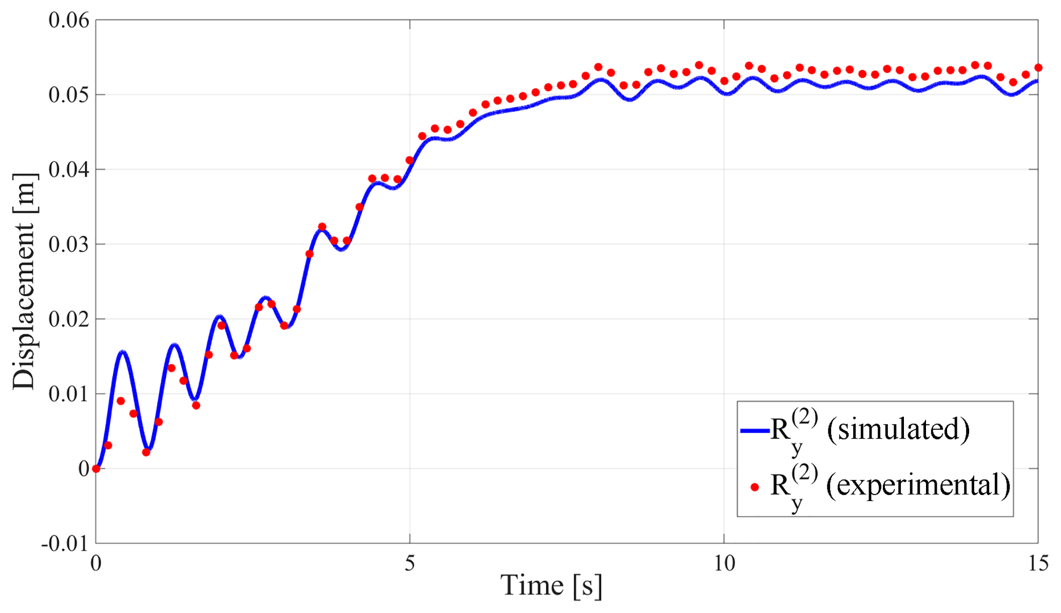
Figure 7 shows the comparison between the simulation of transverse displacement ${\mathbf{R}}_y^{\left(\mathrm{2}\right)}$ of the nacelle and the experimental data. The working parameters are as follow: twist angle $\mathit{\beta }=\mathrm{25}{}^{\circ }$, wind speed v₂=8 m s⁻¹, three modes to describe the movement of the tower, and six 3-D beam element to construct each blade model. The convergence between the two curves indicates the validity of the selected modal coordinates of the tower and the overall mathematical model of the wind turbine system.

Moreover, the comparisons between the output rotor velocity of the FFR model and the experimental benchmark are shown in Figs. 8 and 9. In these figures, one more curve is added to the work resented in Nada and Al-Shahrani (2017), in which the Nacelle is attached to the tower and the dynamic of both of these two bodies are not included in the model ,i.e. assumed fixed. Figures 8 and 9 show that the experimental and computational results of the model including the tower and Nacelle, coincide with each others to a large extent. It is clear that the source of error mentioned in Nada and Al-Shahrani (2017) was due to the effect of tilting angle of the rotor. Ignoring the effect of this angle results in wrong estimate of the angle of twist of blade as well as the drag force along the rotor blades.

It is concluded that the comparison show a very good agreement which encourage to utilize the wind-turbine model based on the FFR formulation and by using the suggested mixed coordinates model.

5 Conclusions

In this paper, an efficient procedure is developed based on Floating Frame of Reference formulation (FFR) for modeling a complete system components of wind turbine. The dynamic of the tower, nacelle, rotor and blades are included with different sets of coordinates. Modal coordinates are assigned for the tower body, Cartesian coordinates set are assigned for the nacelle and the rotor, and elastic nodal coordinates sets are used for the rotating blades.

The paper describes an experimental test-rig of small size wind turbine in front of wind velocity of 8 m s⁻¹ and the measured rotor velocities are collected and compared with the FFR dynamic model. The experimental work show a very good agreement of the mixed sets model. The results encourage to utilize the wind-turbine model based on the FFR formulation and by using the suggested mixed coordinates for design process, identification and health monitoring aspects. Although the model has been drafted in general form, but it is very important to verify each system under its operating conditions. The authors look forward to applying the proposed method in modeling other applications such as the vertical and large-size wind turbines, helicopters and epicyclic gearboxes.

Appendix A: Shape function matrix

A beam element of 12 degrees of freedom, assuming that the element displacements in the x−y plan and x−z plan are polynomials of third degree and all others are assumed to be linear; the matrix [S]^T can be expressed as:

$$\left[\begin{array}{ccc}\mathrm{1}-\mathit{\xi }& \mathrm{0}& \mathrm{0}\\ \mathrm{6}\left(\mathit{\xi }-{\mathit{\xi }}^{\mathrm{2}}\right)\mathit{\eta }& \mathrm{1}-\mathrm{3}{\mathit{\xi }}^{\mathrm{2}}+\mathrm{2}{\mathit{\xi }}^{\mathrm{3}}& \mathrm{0}\\ \mathrm{6}\left(\mathit{\xi }-{\mathit{\xi }}^{\mathrm{2}}\right)\mathit{\zeta }& \mathrm{0}& \mathrm{1}-\mathrm{3}{\mathit{\xi }}^{\mathrm{2}}+\mathrm{2}{\mathit{\xi }}^{\mathrm{3}}\\ \mathrm{0}& -\left(\mathrm{1}-\mathit{\xi }\right)\mathrm{\ell }\mathit{\zeta }& \left(\mathrm{1}-\mathit{\xi }\right)\mathrm{\ell }\mathit{\eta }\\ \left(\mathrm{1}-\mathrm{4}\mathit{\xi }+\mathrm{3}{\mathit{\xi }}^{\mathrm{2}}\right)\mathrm{\ell }\mathit{\zeta }& \mathrm{0}& \left(-\mathit{\xi }+\mathrm{2}{\mathit{\xi }}^{\mathrm{2}}-{\mathit{\xi }}^{\mathrm{3}}\right)\mathrm{\ell }\\ \left(-\mathrm{1}+\mathrm{4}\mathit{\xi }-\mathrm{3}{\mathit{\xi }}^{\mathrm{2}}\right)\mathrm{\ell }\mathit{\eta }& \left(\mathit{\xi }-\mathrm{2}{\mathit{\xi }}^{\mathrm{2}}+{\mathit{\xi }}^{\mathrm{3}}\right)\mathrm{\ell }& \mathrm{0}\\ \mathit{\xi }& \mathrm{0}& \mathrm{0}\\ \mathrm{6}\left(-\mathit{\xi }+{\mathit{\xi }}^{\mathrm{2}}\right)\mathit{\eta }& \mathrm{3}{\mathit{\xi }}^{\mathrm{2}}-\mathrm{2}{\mathit{\xi }}^{\mathrm{3}}& \mathrm{0}\\ \mathrm{6}\left(-\mathit{\xi }+{\mathit{\xi }}^{\mathrm{2}}\right)\mathit{\zeta }& \mathrm{0}& \mathrm{3}{\mathit{\xi }}^{\mathrm{2}}-\mathrm{2}{\mathit{\xi }}^{\mathrm{3}}\\ \mathrm{0}& -\mathrm{\ell }\mathit{\xi }\mathit{\zeta }& \mathrm{\ell }\mathit{\xi }\mathit{\eta }\\ \left(-\mathrm{2}\mathit{\xi }+\mathrm{3}{\mathit{\xi }}^{\mathrm{2}}\right)\mathrm{\ell }\mathit{\zeta }& \mathrm{0}& \left({\mathit{\xi }}^{\mathrm{2}}-{\mathit{\xi }}^{\mathrm{3}}\right)\mathrm{\ell }\\ \left(\mathrm{2}\mathit{\xi }-\mathrm{3}{\mathit{\xi }}^{\mathrm{2}}\right)\mathrm{\ell }\mathit{\eta }& \left(-{\mathit{\xi }}^{\mathrm{2}}+{\mathit{\xi }}^{\mathrm{3}}\right)\mathrm{\ell }& \mathrm{0}\end{array}\right]$$

such that the non-dimensional quantities, $\mathit{\xi },\mathit{\eta },\mathit{\zeta }$ are defined as: $\mathit{\xi }=x/L$, $\mathit{\eta }=y/L$, $\mathit{\zeta }=z/L$. where L is the length of the element.