A data-driven dynamic modeling method for servo actuators

Servo actuators are widely used in fields such as aerospace, manufacturing, and robotics. Nonlinear factors, including friction, backlash, and transmission error, significantly affect their servo performance. Traditional modeling methods for these nonlinear factors rely on simplified analytical models, which struggle to meet the increasing demands for dynamic model accuracy in control systems. Therefore, this study proposes a data-driven modeling method for nonlinear factors. A back propagation (BP) neural network is employed to perform nonlinear regression analysis of friction and backlash. Based on order spectrum analysis and the principle of dominant order invariance, a multi-order harmonic superposition model is established to describe transmission error. The proposed modeling method has been experimentally validated and demonstrates significantly improved accuracy in nonlinear modeling. Compared with traditional models, the developed data-driven model achieves a goodness of fit exceeding 0.92 with the actual system, an average improvement of over 7 %. Moreover, it accurately captures velocity fluctuations caused by transmission errors, velocity dead zones induced by friction, dynamic backlash variations under load, and uneven friction torque at the same velocity. The proposed data-driven dynamic modeling method can provide valuable insights for accurate modeling of servo systems and controller design.

1 Introduction

Servo actuators equipped with precision reducers such as rotary vector (RV) reducers and harmonic reducers as transmission devices are widely used in fields like aerospace, weapons, robot systems, and manufacturing. Currently, this type of mechanical system is evolving towards higher precision, dynamics, and reliability, and there is significant focus on enhancing the control precision of servo actuators (Zhen et al., 2021). Accurately describing the dynamic characteristics of servo actuators is fundamental to addressing these issues. However, due to the intricacies of nonlinear factors like friction and backlash, the accuracy of the nonlinear models produced by traditional modeling techniques falls short of meeting the demands of the control system. This has long-term adverse impacts on the design of high-precision controllers for servo actuators. Consequently, there is an urgent need to utilize novel principles and methods to achieve more precise dynamic modeling of servo actuators.

Dynamic modeling serves as a crucial approach for addressing practical challenges such as high-precision controller design, state monitoring, and safety control (Chen et al., 2023; Wang et al., 2024; Shi et al., 2025; Xie et al., 2025). Owing to the coupling effects of internal nonlinear factors within transmission components and the system state, the system input and output exhibit highly complex nonlinear dynamic behavior (Margielewicz et al., 2019). Accurately capturing the time-varying nonlinear characteristics of transmission components poses a significant challenge in dynamic modeling. The analytical model of nonlinear factors provides vital support for the dynamic model and plays a pivotal role in enhancing model accuracy. However, given the complexity and feasibility of the model, several simplifications have been made to the nonlinear modeling. For instance, friction is simplified as a Stribeck curve that solely depends on speed (Wang et al., 2024; Guo et al., 2026), backlash is simplified as a dead zone with a fixed size (Sun et al., 2021), and transmission error is simplified as a combination of third-order harmonics (Guo et al., 2023). The simplified modeling approach, which relies on analytical equations to approximate nonlinear factors, struggles to accurately capture the dynamic evolution of nonlinear characteristics in response to changes in the system state.

Currently, data-driven methods based on artificial neural network algorithms have gradually emerged as a research trend for describing nonlinear factors (Brunton and Kutz, 2019). Scholars both domestically and internationally have applied this approach to model the nonlinear characteristics of various systems, including maglev vehicles (Liu et al., 2025), microwave devices (Liu et al., 2024), autonomous vehicles (Cheng et al., 2025), industrial robots (Yang et al., 2025), two-wheeled robots (Khan et al., 2022), and robotic manipulators (Polydoros et al., 2015; Ren and Ben-Tzvi, 2020). These studies have accurately predicted output responses under different input conditions. The data-driven approach has been verified to possess strong nonlinear modeling capabilities. However, the aforementioned modeling methods treat the research object as a black box and rely heavily on the comprehensiveness of experimental data for accurate prediction (Rane et al., 2019).

Adding prior knowledge to the black box model to form a gray box or hybrid model effectively enhances the extended attributes of the model, allowing for easier creation of data-driven models (Hashemi et al., 2023). A hybrid model is a data-driven modeling approach that focuses solely on nonlinear factors within a system, based on its dynamic characteristics. In terms of modeling the backlash and transmission error of transmission components, Wang et al. (2015) applied a back propagation (BP) neural network to describe the relationship between backlash and spindle position in establishing the backlash model in a ball screw kinematic pair and accurately predicted the forward backlash and the reverse backlash. Additionally, Li et al. (2020) considered the nonlinear relationship in which backlash becomes larger with an increase in running time on this basis and used a deep belief network to establish the mapping relationship between backlash, spindle position, and running time, realizing the hierarchical diagnosis and prediction of backlash. Sakaridis et al. (2023) established a symmetry-preserving neural network model for static transmission error of spur gear, with an average prediction error of 0.075 % beyond the training data, realizing high-accuracy prediction of transmission error.

In the nonlinear modeling of friction based on neural network algorithms, friction is reduced to a function of velocity in systems such as industrial robots (Hu et al., 2025), industrial robotic joints (Trinh et al., 2023), and geared transmissions (Hirose and Tajima, 2017), and different neural network algorithms are used to model the static nonlinearity of friction. Tu et al. (2019) considered the relationship between friction and heavy torque when modeling the friction of robotic arm joints, and they applied a BP neural network to establish a mapping relationship between friction, velocity, and heavy torque. Baş and Karabacak (2023a, b) modeled the friction of a cam mechanism and plain bearing respectively using three machine learning algorithms – namely an artificial neural network, a support vector machine, and Gaussian process regression analysis – in which the effects of speed and load on friction were taken into consideration, and proved that the machine-learning-based model can effectively estimate changes in friction torque.

The research mentioned above has primarily focused on nonlinear factors that are challenging to model in transmission systems. By utilizing data-driven methods, nonlinear models such as friction and backlash can be captured effectively. In terms of model accuracy and prediction performance, these data-driven modeling approaches have been shown to possess significant potential in replacing traditional modeling techniques. There are still two issues in the data-driven modeling of servo actuators: first, only the most significant nonlinear factors are considered when modeling the system; second, the model structure is oversimplified when modeling these nonlinear factors. Therefore, there remains considerable room for improving the accuracy of data-driven models for servo actuators.

In this paper, a hybrid modeling method for servo actuators is developed based on the data-driven method. The method integrates nonlinear factor models of friction, backlash, and transmission error into the linear mechanism model of the system. A BP neural network is utilized to establish the mapping relationships between friction, angular velocity, and angular position, as well as between backlash, load torque, and angular position. Furthermore, based on the order-ratio spectral analysis of transmission error and the principle of invariance of the main order, a harmonic superposition model of transmission error is established. Finally, to demonstrate the effectiveness of the proposed method, a specific servo actuator is selected as the research object, and simulations and experiments are conducted to verify the accuracy and versatility of the proposed modeling method.

The article is organized as follows. Section 2 proposes a data-driven servo actuator modeling method. Section 3 constructs a nonlinear factor model for the servo actuator. Section 4 verifies the accuracy of the model through a simulation and an experiment. Section 5 concludes the research work.

2 Dynamic modeling method

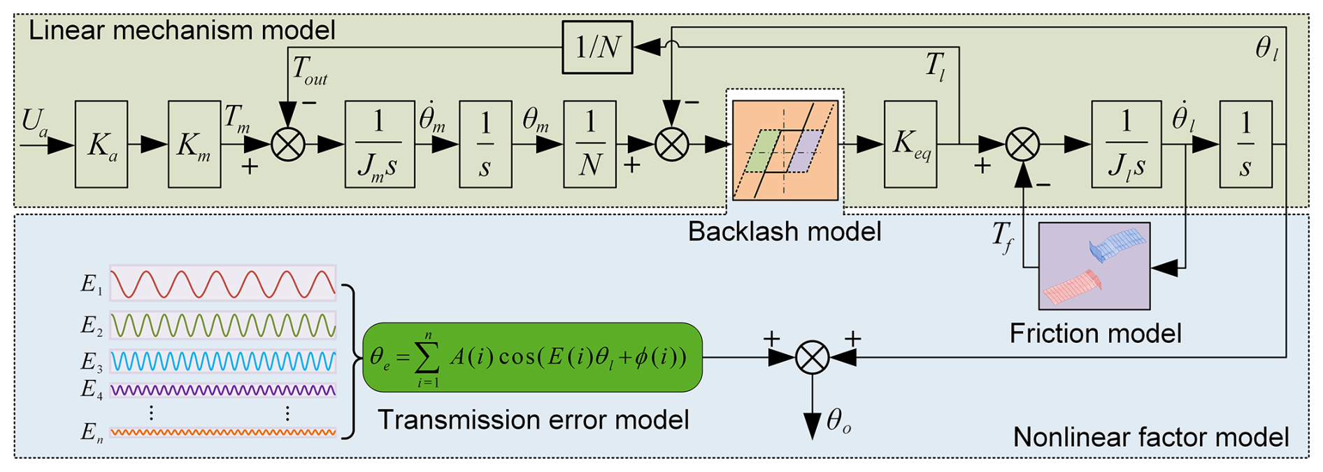
The dynamic modeling method for servo actuators proposed in this paper comprises two main components. Firstly, based on the mechanism of electric–magnetic force–motion changes within the actuator, linear features reflecting the force–displacement relationship are extracted to establish a linear mechanism model of the servo actuator. Subsequently, by analyzing the nonlinear factors that significantly impact servo performance and utilizing data-driven methods to investigate the mapping relationship between nonlinear factors, such as friction, backlash, and transmission error, with system state, a nonlinear factor model of servo actuators is established.

2.1 Linear mechanism modeling

The linear mechanism model is derived by analyzing the mechanisms of electromagnetic conversion, force balance, and displacement changes within the actuator. This model describes the operating state of the system using mathematical tools, such as differential equations and transfer functions, to reflect the linear characteristics of the actuator, and it also reflects the dynamic and kinematic characteristics of most servo mechanisms. The response model of the armature current of the motor to the control command is approximated using a proportional coefficient, while the stiffness coefficient is used to characterize the connection stiffness from the output end of the motor to the load end. Therefore, the servo actuator can be equivalently represented as a dual-inertia dynamic model, and the differential equation of motion is accordingly derived as

$$\begin{array}{}\text{(1)}& \left\{\begin{array}{l}{J}_{\mathrm{m}}{\ddot{\mathit{\theta }}}_{\mathrm{m}}=T_{\mathrm{m}}-T_{\mathrm{out}}\\ J_{\mathrm{l}}{\ddot{\mathit{\theta }}}_{\mathrm{l}}=T_{\mathrm{l}}\\ T_{\mathrm{m}}=K_{\mathrm{a}}{K}_{\mathrm{m}}{U}_{\mathrm{a}}\\ T_{\mathrm{l}}=K_{\mathrm{eq}}\left(\frac{{\mathit{\theta }}_{\mathrm{m}}}{N}-{\mathit{\theta }}_{\mathrm{l}}\right)\\ T_{\mathrm{out}}=\frac{T_{\mathrm{l}}}{N}\end{array}\right.,\end{array}$$

where J_m and J_l are the motor rotor inertia and equivalent load inertia, θ_m and θ_l are the angular position of the motor and load, T_m is the motor output torque, T_l is the torque transmitted to the load by the system, N is the transmission ratio of the reducer, K_eq is the equivalent stiffness coefficient of the system, T_out is the load torque on the motor, U_a is the input voltage of the motor, K_a is the voltage conversion factor of the driver, and K_m is the motor moment coefficient.

Equation (1) can be further simplified as

$$\begin{array}{}\text{(2)}& \left\{\begin{array}{l}{J}_{\mathrm{m}}{\ddot{\mathit{\theta }}}_{\mathrm{m}}=K_{\mathrm{a}}{K}_{\mathrm{m}}{U}_{\mathrm{a}}-K_{\mathrm{eq}}\left(\frac{{\mathit{\theta }}_{\mathrm{m}}}{N}-{\mathit{\theta }}_l\right)/N\\ J_{\mathrm{l}}{\ddot{\mathit{\theta }}}_{\mathrm{l}}=K_{\mathrm{eq}}\left(\frac{{\mathit{\theta }}_{\mathrm{m}}}{N}-{\mathit{\theta }}_{\mathrm{l}}\right)\end{array}\right..\end{array}$$

By presenting the above equation in block diagram form, the linear mechanism model of the servo actuator can be obtained.

2.2 Friction and backlash modeling

In response to the shortcomings of the Stribeck model and other dynamic friction models, an implicit function f_T is used to describe the friction torque based on its correlation with angular velocity and position.

$$\begin{array}{}\text{(3)}& T_{\mathrm{f}}=f_T\left({\mathit{\theta }}_{\mathrm{l}},{\dot{\mathit{\theta }}}_{\mathrm{l}}\right)\text{sgn}\left({\dot{\mathit{\theta }}}_{\mathrm{l}}\right)\end{array}$$

In response to the limitations of the backlash model, based on the relationship between backlash, load torque, and angular position, the nonlinear variation in backlash is represented by an implicit function f_H.

$$\begin{array}{}\text{(4)}& {\mathit{\theta }}_{\mathrm{h}}=f_{\mathrm{H}}\left({\mathit{\theta }}_{\mathrm{l}},T_{\mathrm{L}}\right)\end{array}$$

The above friction model and backlash model are both in the form of implicit functions. The BP neural network algorithm is used for nonlinear regression analysis. The process of modeling and predicting forward friction using the BP neural network is shown in Fig. 1.

Figure 1 BP neural network modeling and prediction. Forward friction as an example.

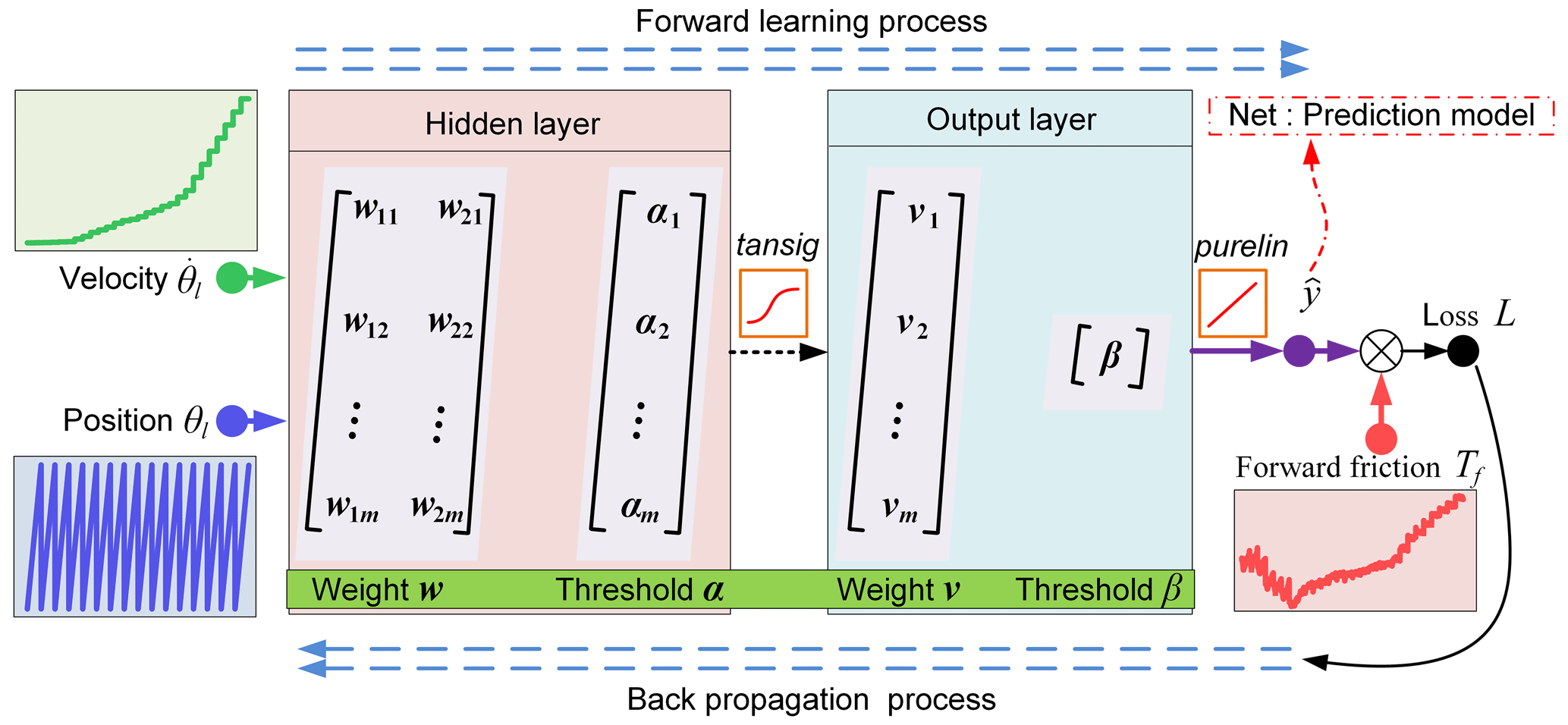
Based on the characteristics of the friction model and the backlash model, a BP neural network with two inputs, one output, and one hidden layer is applied. The input layer nodes are x₁ and x₂, the output layer node is $\widehat{y}$, the number of hidden layer nodes is m, the threshold of the hidden layer is α, the threshold of the output layer is β, the connection weight between the input layer and the hidden layer is w, and the connection weight between the hidden layer and the output layer is v.

After processing the input data x₁ and x₂ through the hidden layer, the output h_j of the hidden layer can be obtained as

$$\begin{array}{}\text{(5)}& h_j=f\left(w_{\mathrm{1}j}{x}_{\mathrm{1}}+w_{\mathrm{2}j}{x}_{\mathrm{2}}-{\mathit{\alpha }}_j\right),j=\mathrm{1},\mathrm{2},\mathrm{\dots }m,\end{array}$$

where f(⋅) is the hidden layer excitation function and defaults to the tansig function.

The output layer output $\widehat{y}$ is

$$\begin{array}{}\text{(6)}& \widehat{y}=g\left(\sum _{j=\mathrm{1}}^m{h}_j{v}_j-\mathit{\beta }\right),\end{array}$$

where g(⋅) is the hidden layer excitation function and defaults to the purelin function.

The loss function is represented by the mean square error (MSE) between the output layer output and the test data, and the loss function L is

$$\begin{array}{}\text{(7)}& L={\displaystyle \frac{\mathrm{1}}{\mathrm{2}}}{\left(T_{\mathrm{f}}-\widehat{y}\right)}^{\mathrm{2}}.\end{array}$$

Assuming the learning factor is η, according to the guiding principle of the gradient descent method, iteratively updating the connection weights w and v, the following expression can be obtained:

$$\begin{array}{}\text{(8)}& \left\{\begin{array}{l}{w}_{ij}(k+\mathrm{1})=w_{ij}\left(k\right)-\mathit{\eta }\frac{\partial L}{\partial w_{ij}},i=\mathrm{1},\mathrm{2},j=\mathrm{1},\mathrm{2},\mathrm{\dots },m\\ v_j(k+\mathrm{1})=v_j\left(k\right)-\mathit{\eta }\frac{\partial L}{\partial v_j},j=\mathrm{1},\mathrm{2},\mathrm{\dots },m\end{array}\right..\end{array}$$

By updating the thresholds using the same method, the updated expressions for thresholds α and β can be obtained:

$$\begin{array}{}\text{(9)}& \left\{\begin{array}{l}{\mathit{\alpha }}_j(k+\mathrm{1})={\mathit{\alpha }}_j\left(k\right)-\mathit{\eta }\frac{\partial L}{\partial {\mathit{\alpha }}_j},j=\mathrm{1},\mathrm{2},\mathrm{\dots },m\\ \mathit{\beta }(k+\mathrm{1})=\mathit{\beta }\left(k\right)-\mathit{\eta }\frac{\partial L}{\partial \mathit{\beta }}\end{array}\right..\end{array}$$

After updating the weights and thresholds each time, we calculate the loss function. When the output of the loss function meets expectations or reaches the upper limit of the iteration, the iteration calculation of the BP neural network ends. If the output of the loss function does not meet expectations, it can be retrained until the result is satisfactory.

2.3 Transmission error modeling

Through the pre-testing and order-ratio spectral analysis of transmission error, the relationship between transmission error and the angular velocity and angular position is described by waveform reconstruction, and the periodic fluctuation in transmission error is expressed by

$$\begin{array}{}\text{(10)}& {\mathit{\theta }}_{\mathrm{e}}=\sum _{i=\mathrm{1}}^{n}A\left(i\right)\cos \left(\mathrm{2}\mathit{\pi }{f}_{\mathrm{te}}\left(i\right){\displaystyle \frac{{\mathit{\theta }}_{\mathrm{l}}}{{\dot{\mathit{\theta }}}_{\mathrm{l}}}}+\mathit{\varphi }\left(i\right)\right),\end{array}$$

where θ_e is the transmission error, f_te is the frequency of transmission error in the angular position domain, A and ϕ are the amplitude and phase of transmission error at frequency f_te respectively, and n is the number of transmission error principal components.

The following commutation relationship exists between the angular position domain frequency f_te and the order E:

$$\begin{array}{}\text{(11)}& E={\displaystyle \frac{\mathrm{2}\mathit{\pi }{f}_{\mathrm{te}}}{{\dot{\mathit{\theta }}}_{\mathrm{l}}}}.\end{array}$$

By associating Eqs. (10) and (11), the transmission error model can be obtained:

$$\begin{array}{}\text{(12)}& {\mathit{\theta }}_{\mathrm{e}}=\sum _{i=\mathrm{1}}^{n}A\left(i\right)\cos \left(E\left(i\right){\mathit{\theta }}_{\mathrm{l}}+\mathit{\varphi }\left(i\right)\right).\end{array}$$

By substituting the order E for the angular position domain frequency f_te, the transmission error model does not contain the angular velocity term of the system, avoiding the influence of velocity noise on the transmission error model.

By modeling the linear mechanism and nonlinear factors such as friction, backlash, and transmission error, the dynamic model diagram of the servo actuator is obtained as shown in Fig. 2.

Figure 2 Block diagram of servo actuator dynamic model.

3 Construction of nonlinear factor model

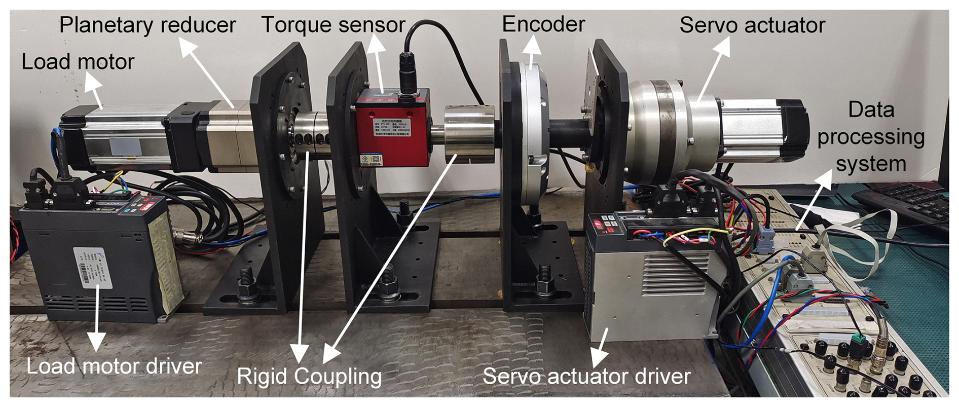
This paper takes a servo actuator as an example and builds the experimental platform shown in Fig. 3. The servo actuator is composed of a permanent magnet synchronous motor (model: ASM80B1007-30M) and an RV reducer (model: ZKRV-20E-161-B). The main components of the experimental platform include an encoder (model: RON-786C), a torque sensor (model: DYN-200), a planetary reducer (model: WAB090-70), and a load motor (model: ASM80B1007-30M). The servo actuator and encoder are connected using the same steel shaft to ensure coaxiality. The load motor, planetary reducer, and torque sensor form a torque closed-loop system, which serves as a load simulation device for the servo actuator. A rigid coupling is used to connect the load simulator and the servo actuator.

Figure 3 Experimental platform.

The nonlinear model is established using the experimental modeling method. Based on the testing methods of friction torque and transmission error, discrete data, such as friction torque, backlash, and transmission error of the servo actuator, are obtained through testing. After preprocessing, the nonlinear factor model can be constructed using the modeling method proposed in Sect. 2, and the model accuracy can be verified.

3.1 Construction of friction model

In the velocity closed-loop mode, the servo actuator is driven to rotate smoothly for one full revolution in both forward and reverse directions from the zero position at different velocities, allowing measurement of the friction torque associated with angular velocity and angular position. The relationship between the friction, velocity, and position is shown in Fig. 4.

Figure 4 The experimental results of friction.

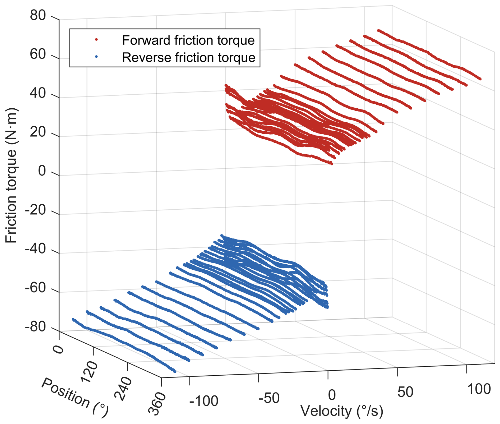
The experimental data under the same velocity command are stored in the form of column vectors, and the column vector datasets under different velocity commands are sequentially combined to form column vector datasets for friction torque, angular position, and angular velocity. Resampling is applied to ensure that the length of the column vectors is consistent across different velocity commands. The resulting datasets are used as inputs and outputs of the BP neural network for training and validation of the friction model. The number of nodes in the hidden layer is set to 30, the learning factor is 0.01, the target error is 10⁻¹², and the maximum number of iterations is 1000.

The MSE, mean absolute error (MAE), and mean absolute percentage error (MAPE) are used as error indicators for the friction model, and the results are shown in Table 1.

Table 1 Error indicators of the friction model.

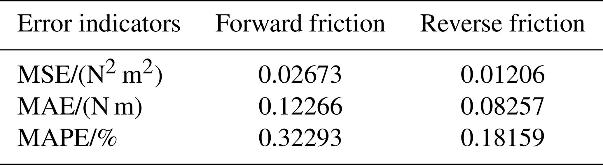
Overall, the validation error of friction torque is very small, distributed within ±1 N m, and the validation error of reverse friction torque is smaller than that of forward friction torque. The MAPE of the validation error of the forward friction model is about 0.32 %, and the MAPE of the validation error of the reverse friction model is about 0.18 %, indicating that the difference between the predicted value and the actual value is small, and the friction model exhibits good performance. The angular velocity and angular position are further refined to verify the convergence of the established friction model at non-test points, and the prediction results of the frictional torque are shown in Fig. 5. The friction at the non-test point continues the relationship between the friction at the test point and the angular velocity and angular position.

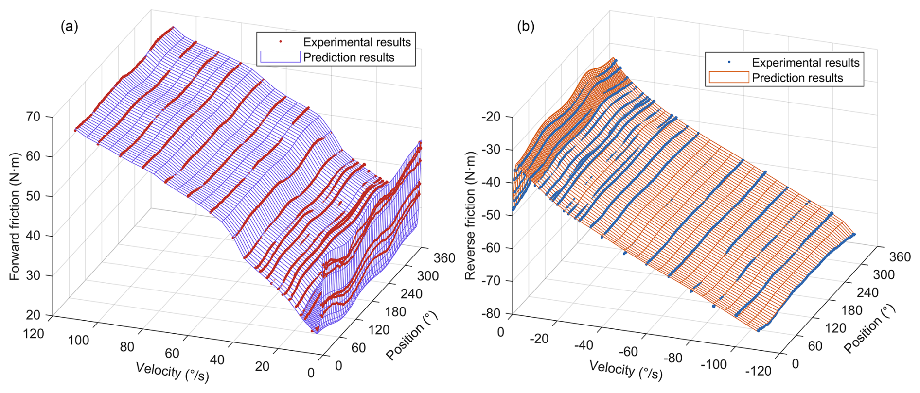
Figure 5 The prediction results of forward friction torque (a) and reverse friction torque (b).

3.2 Construction of backlash model

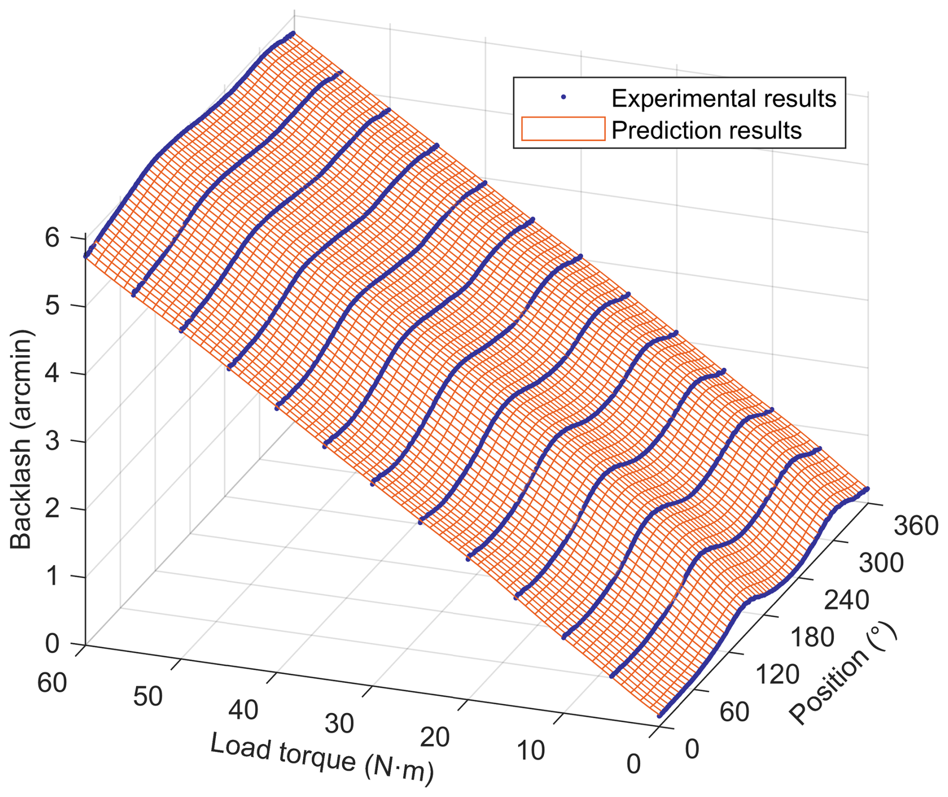
A constant-load torque is applied to the servo actuator, and the bidirectional transmission error of the servo actuator is tested under different load torques in the velocity closed-loop mode. The difference between the forward transmission error and the reverse transmission error is the backlash of the servo actuator. The relationship between backlash, load torque, and angular position is shown in Fig. 6.

Figure 6 Experimental and filter results of backlash.

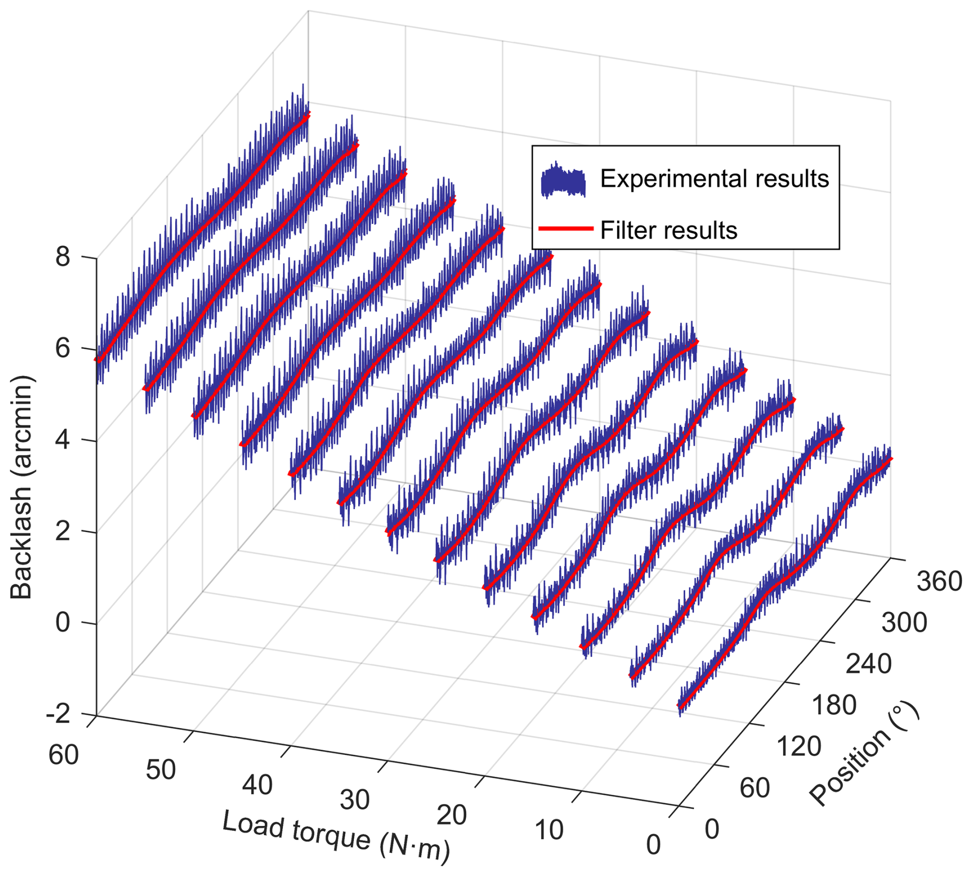
An order spectrum analysis is conducted on the backlash, whose spectral components are the same as the transmission error. To avoid the mutual cancellation of backlash and transmission error due to spectral duplication, the backlash is filtered, and only the low-frequency components are retained, as shown in the filter results represented by the solid red line in Fig. 6. The experimental data of backlash, load torque, and angular position are stored as column vectors and resampled at equal angular intervals to ensure that the three column vectors have the same length. When modeling backlash using the BP neural network, the input layer nodes are the load torque and angular position, the filtered backlash is the output, and other parameter settings are consistent with the friction modeling process. The backlash model is trained and validated, with the error indicators shown in Table 2.

Table 2 Error indicators of the backlash model.

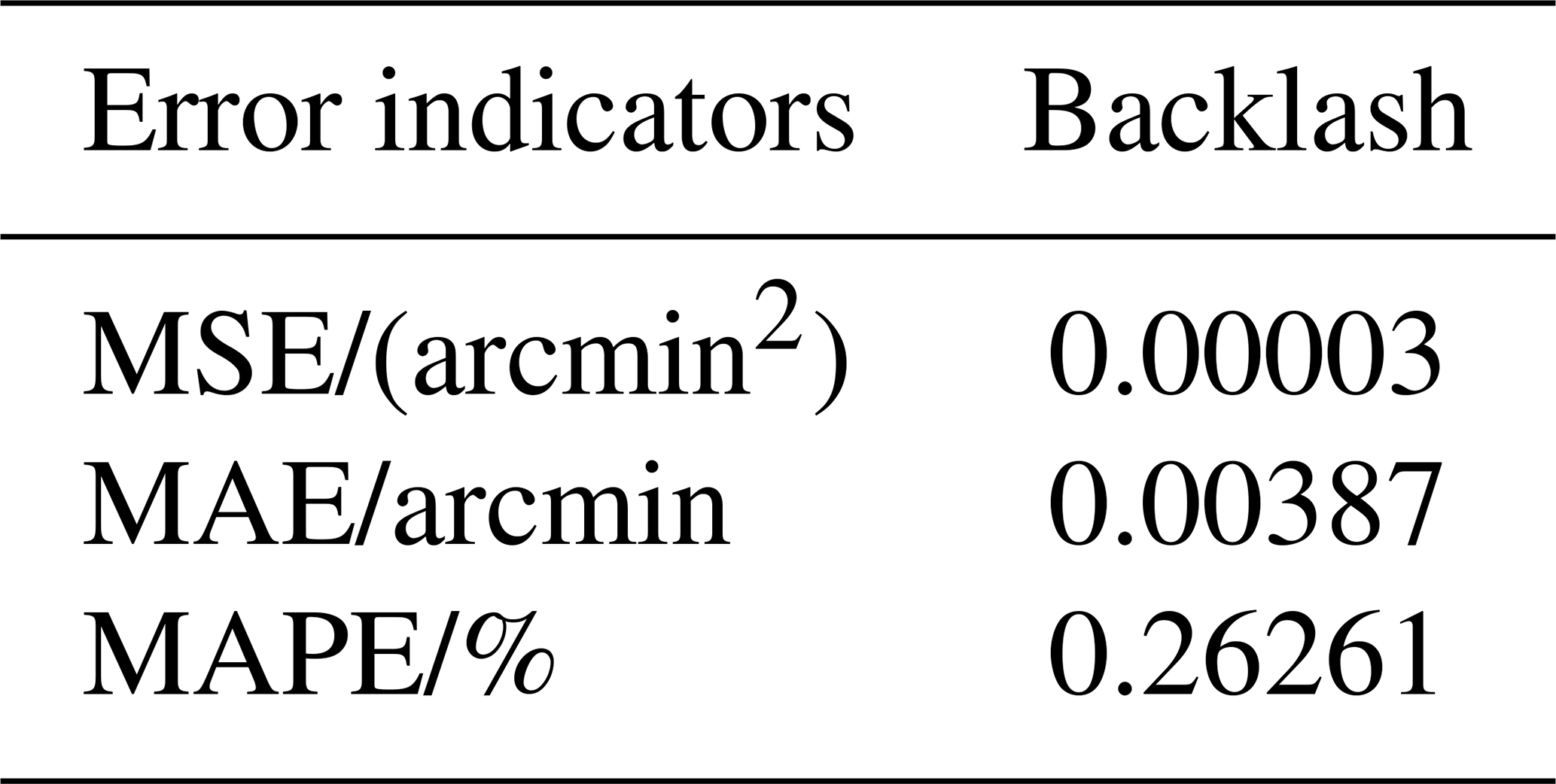
The validation error of the backlash is within ±0.04 arcmin, and the MAPE of the validation results is about 0.26 %, indicating that the backlash model has good fitting performance. The angular position and load torque are further refined to verify the convergence of the established backlash model at non-test points. The predicted results of backlash are shown in Fig. 7. The backlash model fully describes the mapping relationship between backlash, angular position, and load torque. When the load torque is lower, the backlash at different angular positions becomes more uneven.

Figure 7 Prediction results of backlash.

3.3 Construction of transmission error model

In the velocity closed-loop mode, the transmission error of the servo actuator was tested at different velocities, and the relationship between transmission error and angular position is shown in Fig. 8. The order spectrum analysis results of transmission error are shown in Fig. 9.

Figure 8 The experimental results of transmission error.

Figure 9 The order spectrum analysis results of transmission error.

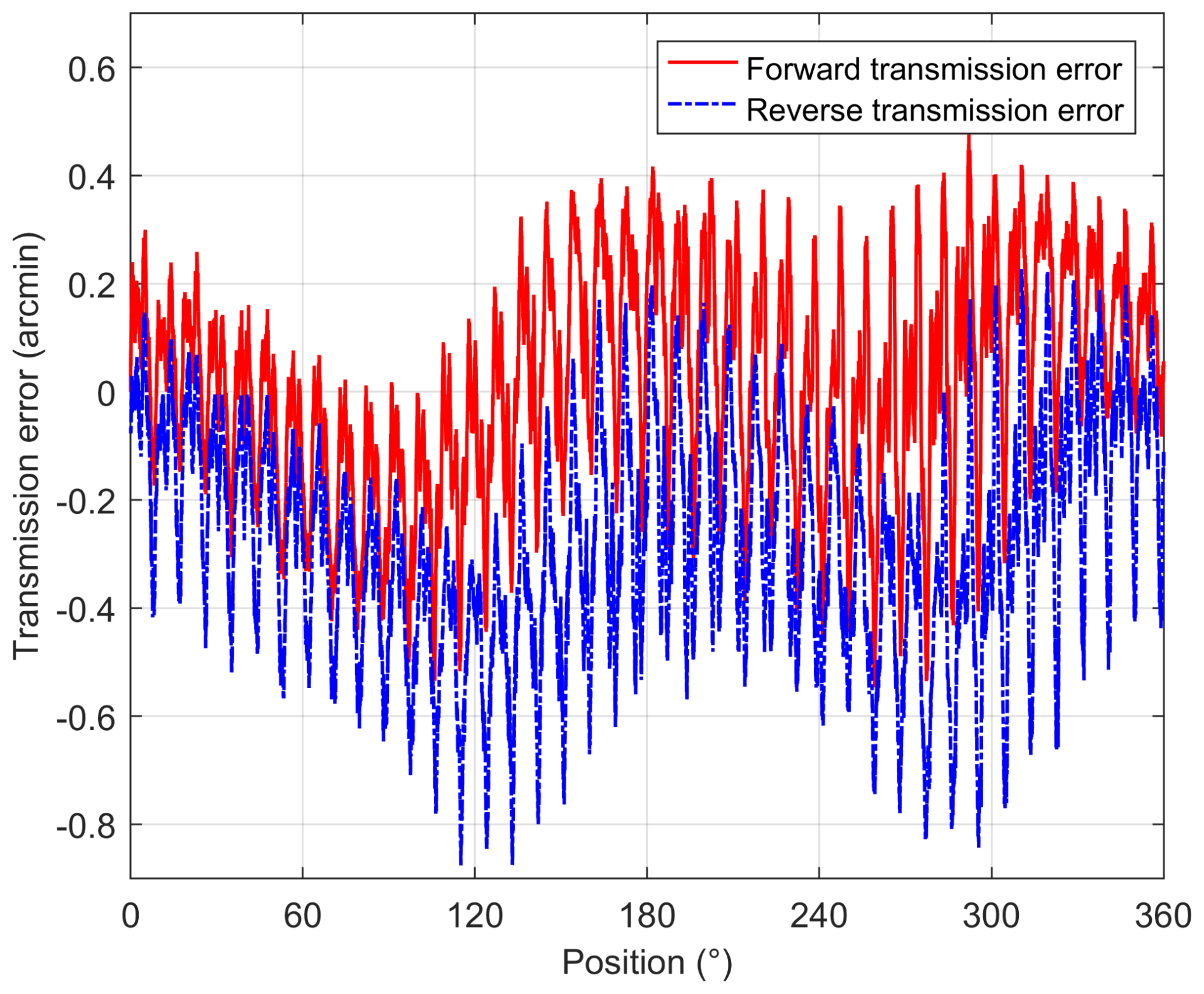
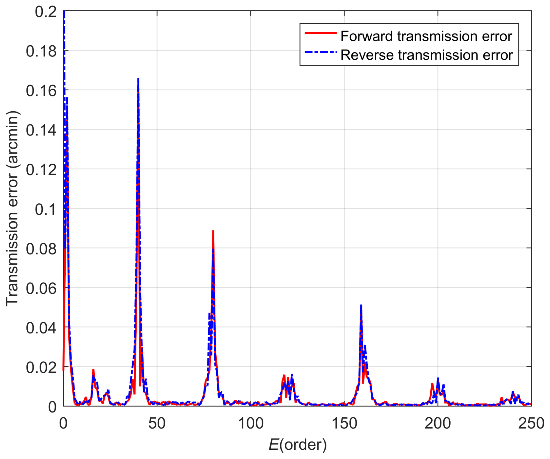
According to the test results and order spectrum analysis results of transmission error, the components of transmission error are mainly concentrated in the 40th order and its multiples, which are related to the periodic meshing of internal gears in precision reducers. By extracting the principal components, order, and phase, the transmission error model of the servo actuator can be constructed according to Eq. (12). The transmission error model is a linear combination of tens of harmonics, preserving the high-frequency components of transmission error. The comparison between the transmission error model and experimental results is shown in Fig. 10. The validation error is basically within ±0.1 arcmin. The MSE of the forward transmission error validation result is only 0.0007314 arcmin², and the MSE of the reverse transmission error validation result is only 0.0016247 arcmin². This indicates that the transmission error model basically coincides with the experimental results, truly describing the transmission error of the servo actuator.

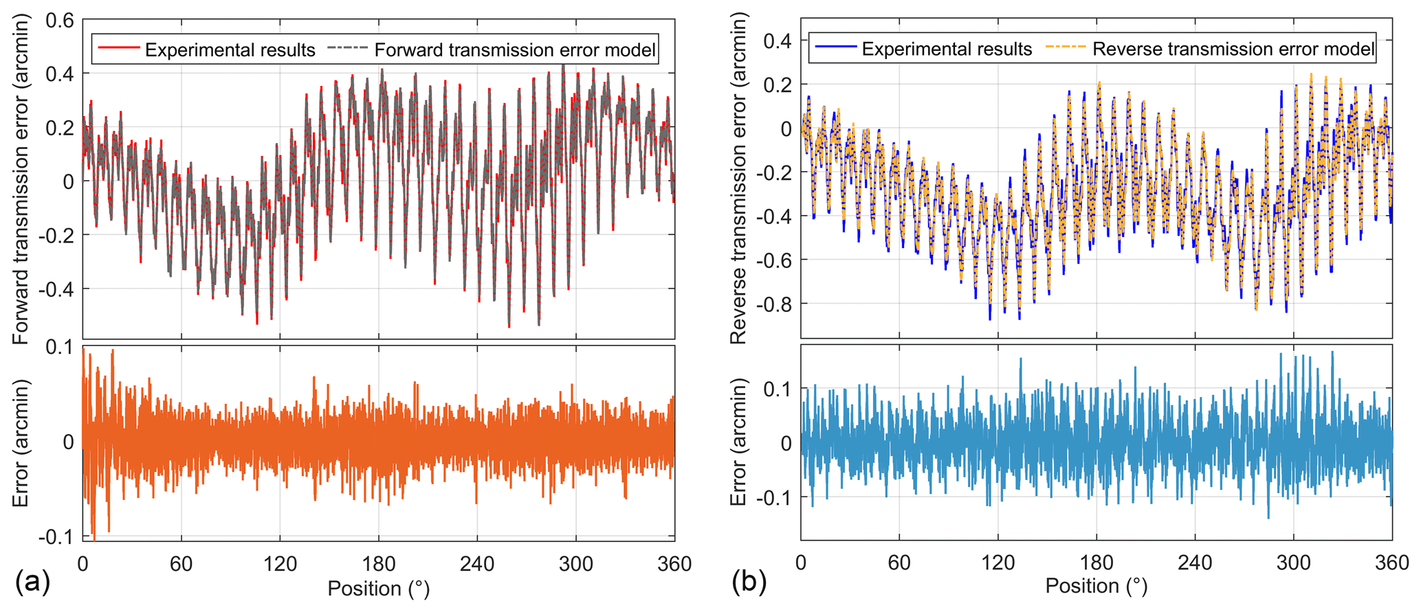
Figure 10 Comparison of experimental results with (a) forward transmission error model and (b) reverse transmission error model.

4 Dynamic model validation

After completing the construction of three nonlinear factor models, along with the linear mechanism model, they collectively form the dynamic model of the servo actuator, referred to as the data model. Compared with a traditional model composed of a linear model, the Stribeck model, a dead-zone model, and a second-order harmonic transmission error model, the data model maximally describes the nonlinear characteristics of the system, which will improve the modeling accuracy of the system to a great extent.

The same velocity controller is employed in both the actual system and the simulation model. The velocity controller adopts a proportional–integral structure, and the detailed design process of these controllers is elaborated on in Jiang et al. (2021), where K_p = 16.09 and K_i = 505.38.

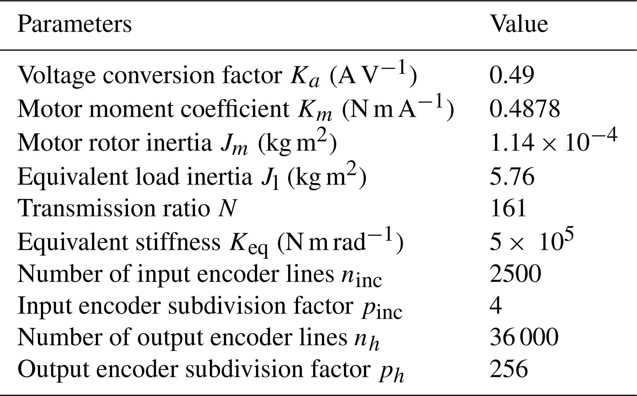
By consulting the product manuals of the servo motor, precision reducer, and encoder, the experimental system parameters shown in Table 3 are obtained. Based on the established servo actuator experimental platform, time-domain response experiments were conducted on the data model, traditional model, and actual system in open-loop, velocity closed-loop, and position closed-loop modes to verify the accuracy of the established data model.

Table 3 The experimental system parameters.

4.1 Open-loop response comparison

In the open-loop mode of the system, the same sinusoidal or square excitation signal is input into the actual system and the simulation model, and the angular velocity of the actual system and the simulation model are recorded and compared to verify the accuracy of the simulation model. Under the excitation of a 1.5 V 1 Hz sine signal, the angular velocity and the velocity error between the simulation model and the actual system are shown in Fig. 11a. The velocity response under the excitation of a 1.8 V 0.5 Hz square signal is shown in Fig. 11b.

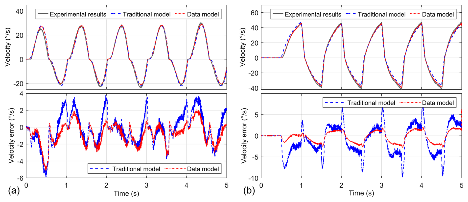
Figure 11 Comparison of time domain response under sine voltage signal (a) and square voltage signal (b).

The angular velocity of the data model is closer to that of the actual system, and the velocity error is obviously smaller than that of the traditional model. The time-domain responses of the sinusoidal and square signals with different amplitudes and frequencies are also tested, and the closeness between the simulation model and the actual system is quantitatively characterized by the goodness of fit in nonlinear regression analysis. The goodness of fit R is calculated as

$$\begin{array}{}\text{(13)}& R=\mathrm{1}-\sqrt{{\displaystyle \frac{\sum {\left(y_i-{\widehat{y}}_i\right)}^{\mathrm{2}}}{\sum y_i^{\mathrm{2}}}}}.\end{array}$$

The closer R is to 1, the closer the fitted data $\widehat{y}$ are to the original data y. Table 4 shows the results of the comparison of the goodness of fit for the angular response.

Table 4 Comparison of goodness of fit for open-loop response.

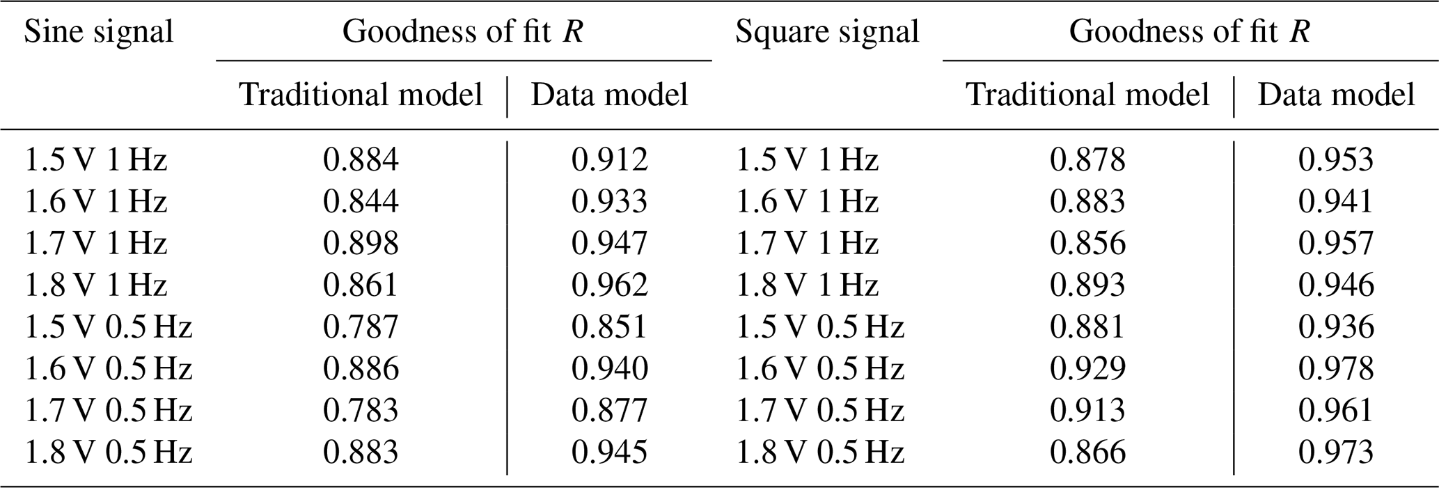
Due to the use of simplified analytical models for nonlinear factors such as friction, backlash, and transmission error in the traditional model, it is not possible to maintain a high goodness of fit over a large range of angular velocity. Compared to the traditional model, the goodness of fit of the sine signal time-domain response in the data model reaches an average of 0.921, an average improvement of 7.3 %, and the goodness of fit of the square signal time-domain response reaches an average of 0.956, an average improvement of 7.1 %.

4.2 Closed-loop response comparison

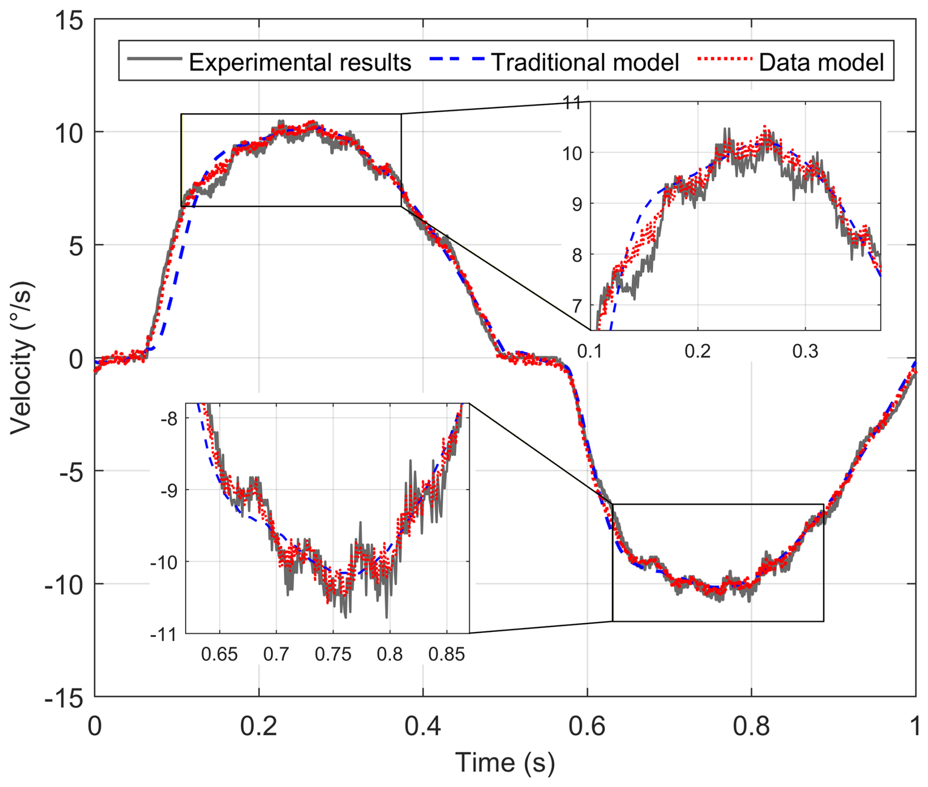
Under the velocity closed-loop mode, the excitation signal is a sinusoidal signal of 10° s⁻¹ 1 Hz, and the angular velocity of the traditional model, the data model, and the actual system are recorded and compared. The comparison of the angular velocity is shown in Fig. 12, which shows that the angular velocity of the traditional model and the data model is basically the same as that of the actual system, and both have the phenomenon of a “dead zone” when the angular velocity passes zero. From the partially enlarged image, the angular velocity of the traditional model is relatively smooth, which is inconsistent with the actual system, while the angular velocity of the data model and the actual system has better consistency and truly reflects the velocity fluctuation phenomenon caused by the transmission error.

Figure 12 Comparison of velocity closed-loop response.

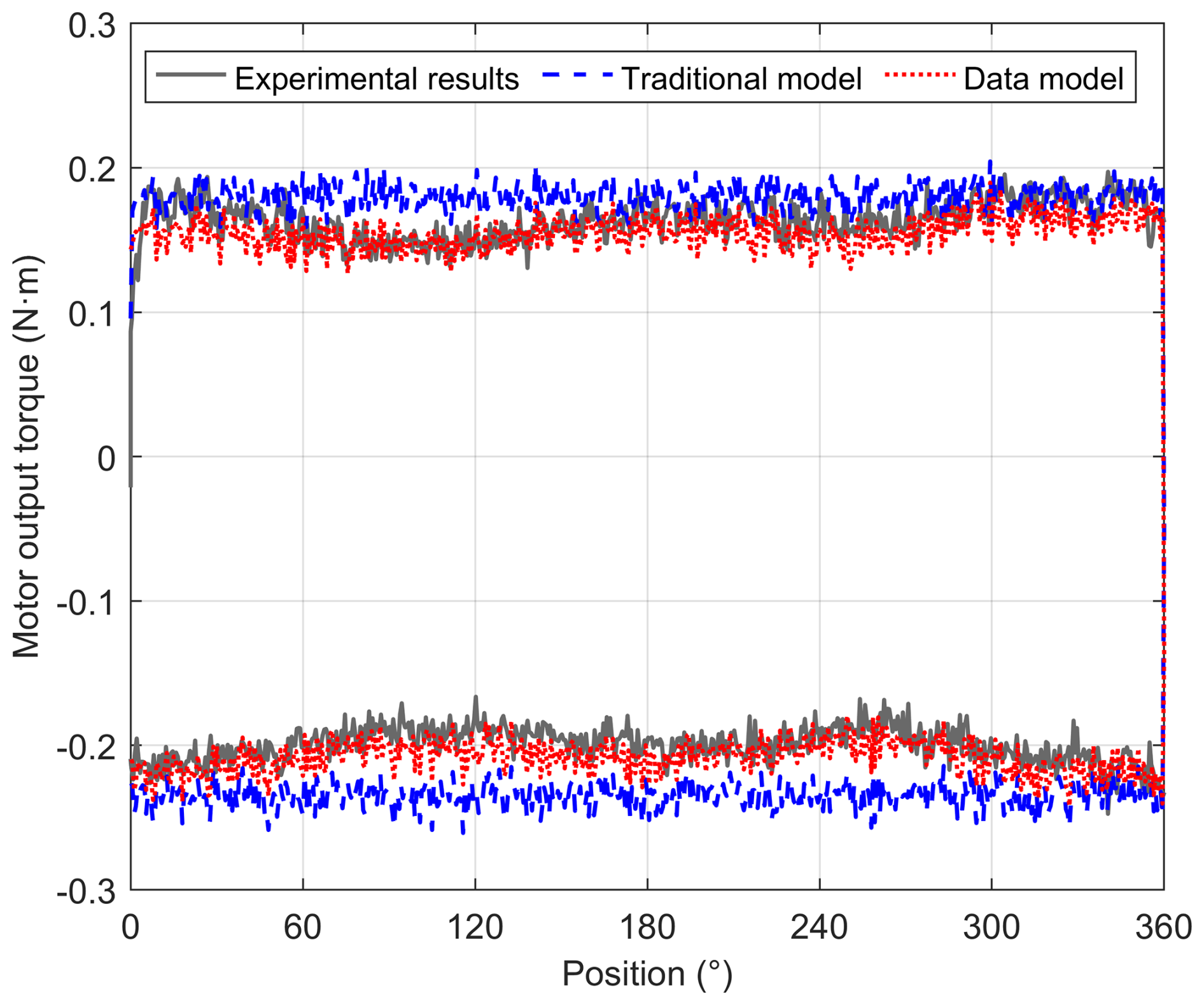
To compare the accuracy of the friction model, under a constant-velocity command of 3° s⁻¹, the motor output torque of the traditional model, data model, and actual system is recorded and compared during one reciprocating cycle over the 360° range of the system. The relationship between the motor output torque and the system angular position is shown in Fig. 13. The change trend of the motor output torque in the data model is basically consistent with the actual system, while the motor output torque of the traditional model basically remains constant, which is very different from the actual system. The relationship between the motor output torque and the angular position reflects the non-uniformity of the friction torque at the output of the system, and compared with the Stribeck model, the friction data model retains this detailed feature, which more realistically reflects the actual system.

Figure 13 Comparison of motor output torque.

In order to compare the effects of different backlash models on the angular position response of the system, backlash tests are conducted under different load conditions according to the definition of backlash. In the position closed-loop mode, a constant load is applied to the output of the system, and the excitation signal is a position ramp signal with a constant slope. When the angular position of the system reaches a certain angle and then reverses the motion, the angular positions of the traditional model, the data model, and the actual system are recorded and compared. The comparison results of the angular position response under different load conditions are shown in Fig. 14.

Figure 14 Comparison of angular position response.

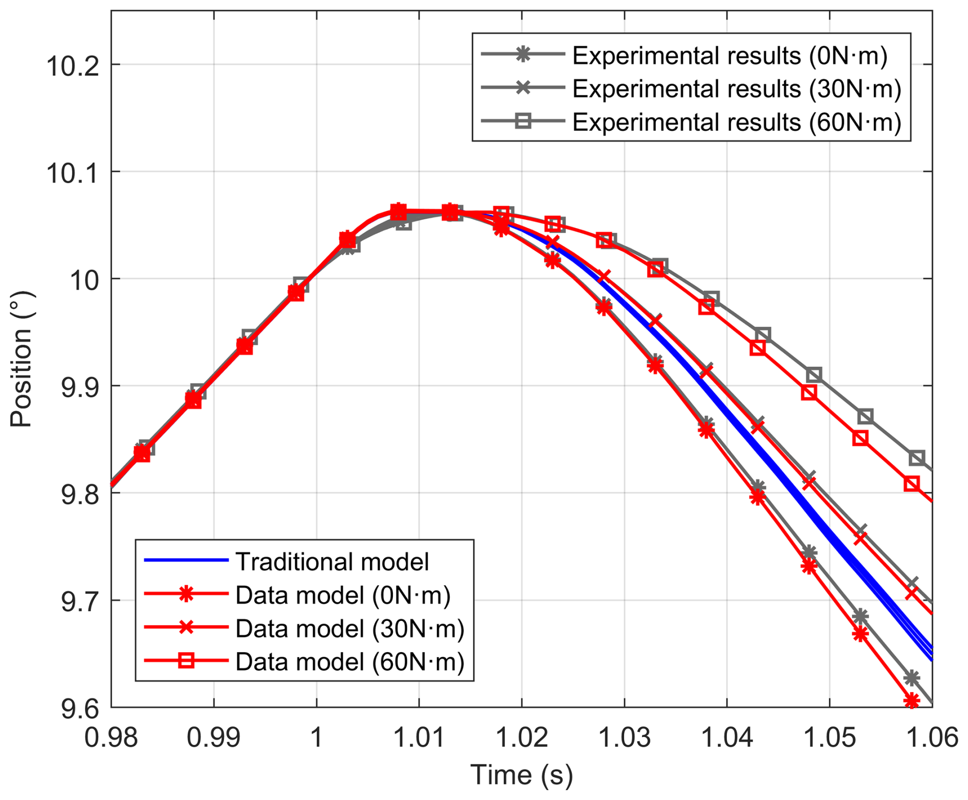
The backlash tests are conducted under 0, 30, and 60 N m load torque to compare the effect of the backlash model on the angular position response of the system. The actual system test values are plotted as solid blue lines, and as the load torque increases, the larger the angular hysteresis and the slower the angular position response as the system changes from forward to reverse rotation. The backlash model with a fixed value is used in the traditional model, ignoring the phenomenon of increasing backlash caused by the load inside the transmission parts. The angular position response curve of the traditional model is shown as a solid green line, and the angular position curves under different load conditions largely overlap, which is a big difference from the actual system. The data model establishes the relationship between backlash and load torque and dynamically adjusts the size of backlash with the change in load torque. The angular position response curve of the data model, marked by the solid red line, has a high degree of agreement with the actual system, which accurately reflects the angular position response of the actual system.

5 Conclusions

Based on data-driven theories and methods, this study successfully constructs a servo actuator dynamic model composed of a linear mechanistic model and a nonlinear factor model. The linear mechanistic model is established through an in-depth analysis of the internal electromagnetic force and motion variation mechanisms within the actuator. To address nonlinear factors such as friction, backlash, and transmission error, a data-driven model for friction and backlash is developed based on a BP neural network, while a transmission error model is built using order spectrum analysis and the principle of dominant order invariance. A series of experimental validations demonstrate the significant effectiveness of the proposed modeling method. Compared with traditional models, the data-driven model achieves a goodness of fit with the actual system exceeding 0.92, representing an average improvement of over 7 %. The model not only accurately reflects velocity fluctuations caused by transmission errors, velocity dead zones induced by friction, and dynamic changes in backlash under varying loads, but also captures uneven friction torque at the same velocity, providing a valuable reference for precise modeling and controller design of servo actuators.

Looking ahead to future research, several promising directions and challenges remain to be explored. Firstly, more complex nonlinear factors should be incorporated to more comprehensively describe the dynamic characteristics of servo actuators. Secondly, further investigation into the time-varying nature of these nonlinear factors is essential, as accurately capturing their temporal evolution is crucial for enhancing model accuracy. Moreover, combining the data-driven model with advanced methods such as online identification and online gradient descent to achieve online updates of the data-driven model, thereby sustainably ensuring the accuracy of the data-driven model under different operating conditions, is also an important direction for future research. At the same time, how to reduce the computational complexity of the model and improve its real-time performance is one of the challenges that need to be overcome.