A novel neural network model for rolling linear guide pair optimization design

This paper addresses the inefficiency of conventional design methods for rolling linear guide pairs, which rely on finite-element analysis and large data demands. This study pioneers a few-shot learning framework based on meta-learning, employing a model-agnostic meta-learning strategy to train an inverted-bottleneck residual fully connected network. The network achieves high prediction accuracy (R²>0.91) with only 126 samples. An integrated parametric platform reduces modelling time from 50 to 2–3 min, significantly improving efficiency. Optimization via sequential least squares quadratic programming demonstrates a 57 % reduction in vertical deformation. However, the current work focuses on static performance optimization, leaving dynamic aspects for future research. This approach offers an efficient and data-effective paradigm for precision mechanical component design.

1 Introduction

The rolling linear guide is a core transmission component in precision mechanical equipment. Its structural performance directly determines the positioning accuracy and service life of high-end equipment, such as computer numerical control (CNC) machine tools and industrial robots (Yang et al., 2020; Wang et al., 2018; Zha et al., 2024; Quan and Zhao, 2024). The traditional guide design method relies much on empirical trial and error (Phuyal et al., 2020; Sahoo and Lo, 2022; Liu et al., 2023; Staroszyk et al., 2024). Designers repeatedly adjust geometric parameters and conduct the computer-aided engineering (CAE) analysis to improve mechanical performance, which is quite time-consuming (Zou and Wang, 2015; Tong et al., 2020). Therefore, a rapid and effective design method should be developed for the structural optimization of a rolling linear guide.

Several studies have been conducted for the investigation of rolling linear guide pairs. For instance, Shimizu (1998) and Ohta and Hayashi (2000) were dedicated to developing rigid models for rolling linear guides based on Hertz contact theory. Cheng (2021) introduced a novel stiffness matrix for roller linear guides, investigating the relationship between non-uniform load distribution and contact states. Xu et al. (2023) developed an analytical dynamic model for flexible linear guides, investigating the vibration behaviour of carriages under external periodic excitations in multiple directions. Compared to numerical analysis methods, the finite-element method (FEM) provides higher computational efficiency and superior adaptability. For example, Sun et al. (2015) established a high-fidelity finite-element model accounting for ball-raceway contact. Wei et al. (2022) used FEM to characterize the impact of structural parameters on guide pair mechanical performance. Tong et al. (2019) employed FEM to develop a 5-degree-of-freedom model for calculating the fully occupied stiffness matrix of linear ball guides. Up until now, few studies have paid attention to the structural optimization of rolling linear guides. In addition, structural optimization design with the results of FEM analysis is quite time-consuming and labour-intensive because FEM analysis cannot directly give the explicit relationships between structure and performance.

Traditional optimization algorithms like PSO and GA are highly effective in handling complex problems. However, they require thousands of computations on high-precision models, and so the cycle is very time-consuming. For example, Tong et al. (2020) employed a particle swarm optimization algorithm, using 2000 particles and running for 150 iterations to optimize the design of the linear guide. Wang et al. (2016) utilized finite-element analysis and a genetic algorithm model, conducting 1580 calculations to optimize the structure of a wind turbine blade. In recent years, machine learning techniques (Ramu et al., 2022) have offered another option for designers. For instance, Kazem et al. (2025) proposed a RAGN-R (surrogate multi-subject ensemble machine learning method) for estimating the mechanical properties of advanced materials. This method can directly establish the connection between structure and performance, enabling highly accurate predictions. Up to now, there have been many types of surrogate models. For instance, Fishwick (1989) used a multi-layer neural network model as a simulation model for a basic ballistic model. Jiang et al. (2025) proposed a multi-fidelity fully connected neural network (FCNN) model to optimize the fin structure of rocket projectiles. Roy et al. (2019) developed a support vector regression (SVR) model for the reliability estimation of engineering structure. Nagendra et al. (2005) developed a response surface model based on the optimal noise, vibration, and harshness (NVH) response sensitivity data for optimizing tailored rolled blank (TRB) components. Machine learning, particularly surrogate models, provides a novel solution for the optimization of rolling linear guide pairs. It directly maps the complex nonlinear relationships between geometric parameters (contact angle and curvature ratio) and mechanical properties (including stiffness and stress). It reduces FEM time from hours to minutes, saving significant iterative computation costs for optimization design.

However, surrogate models typically demand a large number of samples to construct datasets, resulting in substantial computational and workload burdens. To enhance efficiency, it is necessary to reduce sample size requirements without losing the accuracy. Therefore, few-shot learning methods (Huisman et al., 2021) have been developed, possessing strong generalization capabilities, minimal data requirements, and high learning efficiency. Su et al. (2022) developed a novel DRHRML (data reconstruction hierarchical recurrent meta-learning) method for few-shot learning in intelligent bearing fault detection. Liu et al. (2016) proposed a support vector machine (SVM) gait controller trained with limited samples for stable bipedal robotic walking. In the field of few-shot learning, model-agnostic meta-learning (MAML) learns a highly task-sensitive model initialization, enabling rapid adaptation to new tasks with minimal examples (Fallah et al., 2020). To validate the algorithm selection rationale in this study, a comparative analysis was conducted between MAML and other algorithms. Compared to the Reptile algorithm (Nichol and Schulman, 2018), which employs first-order approximations for improved computational efficiency, its predictive accuracy may be inadequate for complex nonlinear regression problems. In contrast, meta-SGD (Li et al., 2017) introduces learnable learning rates, which increases the risk of overfitting when handling extremely small datasets. Transfer learning requires a large and relevant source task, which is often difficult to find in mechanical engineering. Therefore, this study selects MAML for application in the optimization design of rolling linear guide pairs. With only 126 sample sets, it achieves a prediction accuracy with R² exceeding 0.91.

Rolling linear guide pairs serve as core transmission components in precision mechanical equipment. The design and performance metrics must satisfy the stringent requirements of high-end application scenarios. The details are outlined below.

1. High positioning accuracy and motion smoothness. High stiffness and low deformation are core requirements for ensuring precision.

2. High load capacity and long service life. Controlling the maximum contact stress is the key to ensuring service life.

3. High reliability and stability. The design must ensure consistent and predictable performance under various working conditions, preventing performance degradation caused by improper parameter matching.

This paper proposes a meta-learning-based inverted-bottleneck residual fully connected network model. The surrogate models for guide pair stiffness and maximum contact stress were established, and the SLSQP optimization algorithm was employed to solve structural parameter optimization. In addition, this study develops a parametric design platform for guide pairs, which enhances the efficiency of dataset construction through parametric modelling and automated FEM.

The structure of this paper is organized as follows: Sect. 2 establishes the response surface model for predicting the mechanical performance of guide pairs, detailing the few-shot learning process. Section 3 presents the developed parametric modelling platform and couples it with automated FEM, establishing an integrated design–simulation workflow. In Sect. 4, comprehensive analysis of the results is conducted. Finally, Sect. 5 summarizes the study.

2 Meta-learning-based inverted-bottleneck residual fully connected network model

Few-shot learning is a machine learning paradigm that achieves efficient learning with limited training samples. This section integrates the inverted-bottleneck structure with a fully connected network and employs the model-agnostic meta-learning (MAML) algorithm to train this model, achieving rapid cross-task adaptation capability.

2.1 Enhanced Latin hypercube sampling for input sample set construction

To ensure the coverage of the parameter space, a sampling strategy is introduced in this section. The Latin hypercube sampling (LHS) method is employed to ensure a uniform and representative distribution of input samples within the parameter space. In addition, a Euclidean distance constraint is introduced to prevent samples from being excessively close to each other.

Before conducting LHS, the value ranges of all parameters must be normalized to the interval [0,1]. For a raw parameter x_j∈ [a_j,b_j], the normalized value $\stackrel{\mathrm{‾}}{x_j}$ is calculated as follows:

$$\begin{array}{}\text{(1)}& x_j={\displaystyle \frac{x_j-a_j}{b_j-a_j}}.\end{array}$$

Specifically, the value range of each dimension is uniformly divided into N equal subintervals. For each dimension j, a random permutation π_j is generated, where π_j(i) denotes the subinterval number assigned to the i-th sample in the j-th dimension. Based on this, the specific value X_ij for each sample point can be obtained through the following calculation:

$$\begin{array}{}\text{(2)}& {\mathit{X}}_{ij}={\displaystyle \frac{{\mathit{\pi }}_j\left(i\right)-{\mathit{u}}_{ij}}{N}},\end{array}$$

where u_ij is a random number sampled from the uniform distribution U(0,1). Following LHS sampling, the parameters must undergo de-normalization processing, linearly mapping X_ij from [0,1] to the actual parameter range [a_j,b_j] for each variable:

$$\begin{array}{}\text{(3)}& {\mathit{S}}_{ij}=a_j+\left(b_j-a_j\right)\cdot {\mathit{X}}_{ij},\end{array}$$

where S_ij denotes the actual parameter values output by the final Latin hypercube sampling. When adding new samples, a new sample point must not lie too close to any existing samples to avoid spatial clustering and data redundancy. Therefore, when adding new samples, a Euclidean distance (Parhizkar, 2015) is introduced to ensure sample dispersion:

$$\begin{array}{}\text{(4)}& D_{\mathrm{g}}\left(\mathit{p}\mathbf{,}\mathit{X}\right)=\begin{array}{c}min\\ k=\mathrm{1},\mathrm{\dots }N\end{array}\parallel \mathit{p}-{\mathit{x}}_k{\parallel }_{\mathrm{2}}>{\mathit{\delta }}_{\mathrm{g}},\end{array}$$

where p denotes the new candidate sample, X represents the set of existing samples, N indicates the sample count, $\parallel \cdot \parallel \mathrm{2}$ is the Euclidean norm, and δ_g=0.5 denotes the global distance threshold. The global threshold δ_g=0.5 was set based on empirical rules commonly used in experimental design. This setting aims to ensure a sufficient minimum Euclidean distance between sample points in the normalized parameter space. It effectively prevents sample clustering while guaranteeing spatial-filling properties. However, it should be noted that, for parameters with smaller value ranges (such as the ball-positioning angle θ and the interference fit δ in Sect. 4.2, which have small value ranges), a threshold of 0.5 is evidently excessive and inappropriate. Thus, these parameters should be separately assigned a threshold of δ=0.05.

2.2 Inverted-bottleneck residual fully connected network model

Deep neural networks (DNNs) are a significant branch of artificial neural networks (Sze et al., 2017). This section utilizes a fully connected deep neural network (FCNN). By integrating an inverted-bottleneck structure and residual connections, a novel deep residual multi-layer perceptron (MLP) architecture is developed. The cascade architecture – comprising an input layer, multiple residual blocks, and an output layer – effectively captures nonlinear mappings between rolling linear guide design parameters and mechanical performance.

The structural design of neural networks is a pivotal factor in determining their performance. In traditional bottleneck architectures (e.g. ResNet's Bottleneck), a “wide–narrow–wide” pattern is typically adopted. High-dimensional inputs are compressed into a low-dimensional space for feature extraction and then are expanded back to the original high-dimensional space. In contrast, inverted-bottleneck structures (e.g. MobileNetV2) employ the opposite “narrow–wide–narrow” paradigm: low-dimensional inputs are expanded into a high-dimensional space for feature extraction and then return to low dimensionality (Sandler et al., 2018).

Figure 1 illustrates the dimensional transformation schematic of the bottleneck structure and the inverted-bottleneck structure. The inverted-bottleneck structure overcomes the limitations of feature extraction in low-dimensional spaces. This enables the model to possess stronger representational capabilities and capture higher-level features more readily.

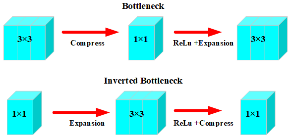
Figure 1 Comparison of dimension transformation with and without inverted-bottleneck structure.

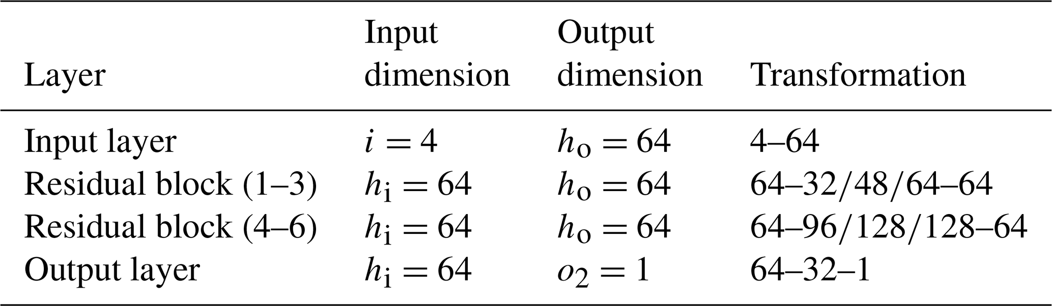
In inverted-bottleneck structures, the ReLU activation function is typically positioned after the dimensionality expansion layer and preceding the compression layer. Its primary role is to introduce nonlinear transformations, enabling the model to learn more complex functions. Without the ReLU function, multiple linear transformations would be equivalent to a single linear transformation, severely limiting the model's representational capacity. Figure 2 depicts the inverted-bottleneck residual fully connected network model (IB-ResFCN) proposed in this study. Table 1 specifies the detailed parameters of the model, which consists of one input layer, six residual blocks, and two regression output layers.

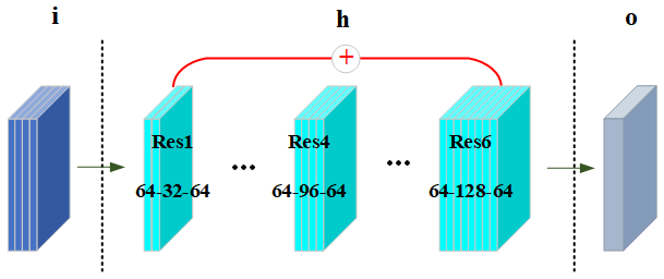
Figure 2 Schematic diagram of the inverted-bottleneck residual fully connected network architecture.

Table 1 Layer parameters of the fully connected neural network.

Residual connections directly link each residual block and effectively prevent gradient vanishing in MLP. Their mathematical expression is as follows:

$$\begin{array}{}\text{(5)}& \mathbf{y}=\mathit{x}+{\sum }_{i=\mathrm{1}}^{\mathrm{6}}F\left(\mathit{x}\right),\end{array}$$

where y denotes the final output, x represents the input, and F(x) signifies the transformation applied to the current input by the network layers.

Residual blocks create a shortcut path, enabling gradients to rapidly back propagate. The first three residual blocks gradually extract higher-dimensional features through progressively increasing dimensions, thereby enhancing the model's expressive capability. The last three residual blocks employ the inverted-bottleneck structure to achieve dimensional expansion, thereby refining the features.

2.3 MAML for supervised learning

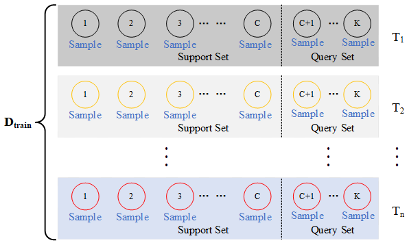
Based on the IB-ResFCN model, meta-learning is applied to enhance prediction accuracy. Meta-learning includes three stages: meta-training, meta-validation, and meta-testing. According to the stages, the dataset is divided into the ratio of training set (D_train) : validation set (D_val) : test set ($D_{\mathrm{test}})=\mathrm{6}:\mathrm{2}:\mathrm{2}$.

Based on distinct task types, meta-learning can be categorized into supervised meta-learning (SML) and meta-reinforcement learning (Meta-RL). Few-shot learning has been extensively researched in the supervised-task domain. Its objective (Finn et al., 2017) is to learn a new function from a limited number of input–output pairs using prior data from similar tasks through meta-learning. This paper employs the model-agnostic meta-learning (MAML) algorithm applied to SML.

In SML, the training set is divided into T meta-tasks, each including K samples. These samples are divided into support and query sets at a 7:3 ratio. Figure 3 illustrates the classification method for the training set. The support set is used for the inner loop, and the query set is used for the outer loop.

Figure 3 Schematic diagram of training-set partitioning.

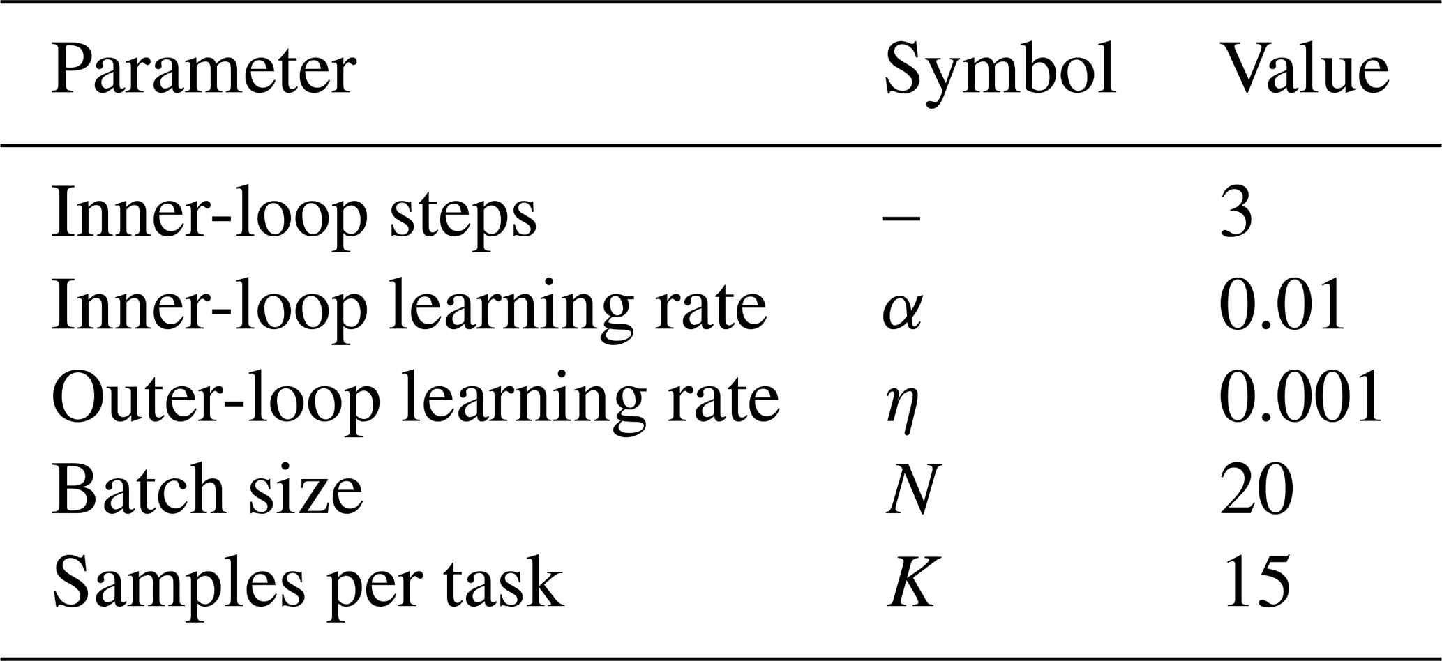
As shown in Fig. 4, at the beginning of the meta-training, three critical parameters are defined: (1) initial meta-parameters θ₀, (2) inner-loop learning rate α and (3) outer-loop learning rate η. Then multiple epochs of meta-training will be conducted. In each epoch, the training set is divided into N meta-tasks: T_i (i=1,2,...,n)∈D_train. Each task is assigned a unique meta-learner M_i and its corresponding initial parameters θ_i. By using the corresponding task T_i, task-specific fast weights ${\mathit{\theta }}_{\mathrm{1}}^{\prime }$ are computed. Subsequently, the gradient ∇ and loss 𝓛 for the current round are computed. Then, the meta-learner for the next round M_i+1 and the parameters θ_i+1 are updated. We repeat the above process until all rounds of meta-training are completed. Finally, the meta-initialization parameters θ_n are acquired. Table 2 shows the parameter settings for MAML training.

Figure 4 Meta-parameter optimization framework for meta-training process.

Table 2 MAML parameter settings.

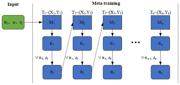
Considering only a single gradient update step, this section explains how θ_i is updated to θ_i+1 in task T_i+1. Based on θ_i and the support set data, ${\mathit{\theta }}_{i+\mathrm{1}}{}^{\prime }$ is computed via gradient descent.

$$\begin{array}{}\text{(6)}& {\mathit{\theta }}_i{}^{\prime }={\mathit{\theta }}_i-\mathit{\alpha }{\mathrm{\nabla }}_{\mathit{\theta }}{\mathcal{L}}_{\mathrm{S}}\left({\mathit{\theta }}_i\right)\end{array}$$

In the above, ℒ_S represents the loss function of the support set. The purpose of the inner loop is to rapidly adapt the model parameters of the support set. In the query set, the loss ${\mathcal{L}}_Q\left(\mathit{\theta }{{}^{\prime }}_{i+\mathrm{1}}\right)$ is computed using the fast weights ${\mathit{\theta }}_{i+\mathrm{1}}^{\prime }$:

$$\begin{array}{}\text{(7)}& {\mathrm{\nabla }}_{\mathit{\theta }}{\mathcal{L}}_Q\left(\mathit{\theta }{{}^{\prime }}_{i+\mathrm{1}}\right)={\displaystyle \frac{\mathit{\delta }{\mathcal{L}}_Q\left(\mathit{\theta }{{}^{\prime }}_{i+\mathrm{1}}\right)}{\mathit{\delta }\mathit{\theta }{{}^{\prime }}_{i+\mathrm{1}}}}\cdot {\displaystyle \frac{\mathit{\delta }\mathit{\theta }{{}^{\prime }}_{i+\mathrm{1}}}{\mathit{\delta }{\mathit{\theta }}_i}}.\end{array}$$

Through the chain rule, the relation of $\mathit{\theta }{{}^{\prime }}_{i+\mathrm{1}}$ in θ_i is incorporated into the gradient computation. Based on this, we update θ_i to θ_i+1:

$$\begin{array}{}\text{(8)}& {\mathit{\theta }}_{i+\mathrm{1}}={\mathit{\theta }}_i-\mathit{\eta }{\mathrm{\nabla }}_{\mathit{\theta }}{\mathcal{L}}_Q\left(\mathit{\theta }{{}^{\prime }}_{i+\mathrm{1}}\right).\end{array}$$

The aim of the outer loop is to optimize θ_i, ensuring that the generated fast weights $\mathit{\theta }{{}^{\prime }}_{i+\mathrm{1}}$ achieve optimal performance in the query set. After N task iterations, the final meta-initial parameters θ_n can be calculated.

$$\begin{array}{}\text{(9)}& \begin{array}{c}\text{min}\\ \mathit{\theta }\end{array}{\sum }_{i=\mathrm{1}}^n{\mathcal{L}}_Q\left({\mathit{\theta }}_i\right)={\sum }_{i=\mathrm{1}}^n{\mathcal{L}}_Q\left({\mathit{\theta }}_{i-\mathrm{1}}-\mathit{\alpha }{\mathrm{\nabla }}_{\mathit{\theta }}{\mathcal{L}}_{\mathrm{S}}\left({\mathit{\theta }}_{i-\mathrm{1}}\right)\right)\end{array}$$

$$\begin{array}{}\text{(10)}& {\mathit{\theta }}_n={\mathit{\theta }}_{\mathrm{0}}\mathit{\eta }{\sum }_{i=\mathrm{1}}^n{\mathrm{\nabla }}_{\mathit{\theta }}{\mathcal{L}}_Q\left(\mathit{\theta }{{}^{\prime }}_{\mathrm{I}}\right)\end{array}$$

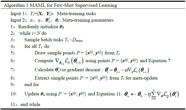
SML can address both classification and regression problems. In regression analysis, a loss function ℒ (θ) is designed to measure the error between predicted outputs and true values. The ℒ (θ) for supervised regression is the mean squared error (MSE), formulated as follows:

$$\begin{array}{}\text{(11)}& \mathcal{L}\left(\mathit{\theta }\right)={\sum }_{x^{\left(j\right)},y^{\left(j\right)}\sim T_i}\mathrm{|}\mathrm{|}{f}_{\mathit{\theta }}\left({\mathit{x}}^{\left(i\right)}\right){\mathit{y}}^{\left(j\right)}\mathrm{|}{\mathrm{|}}_{\mathrm{2}}^{\mathrm{2}},\end{array}$$

where x^(j) and y^(j) denote the input value and the true value of a sample within T_i. Algorithm 1 is the MAML algorithm for supervised learning.

2.4 Fine-tuning phase

The preceding section explained the algorithm for SML and the process of obtaining θ_n. However, θ_n cannot serve as a new starting point for rapid task adaptation of the model. Due to insufficient training samples per meta-task during meta-training, the model fails to adequately learn task-specific patterns. Thus, after meta-training, fine-tuning is performed using the entirety of the training-set samples. This process ensures higher model-learning efficiency. We perform K training iterations on θ_n to update and obtain θ_k:

$$\begin{array}{}\text{(12)}& {\mathit{\theta }}_k={\mathit{\theta }}_{k-\mathrm{1}}{\mathit{\alpha }}_T{\mathbf{\nabla }}_{\mathit{\theta }}{\mathcal{L}}_{\mathrm{train}}\left({\mathit{\theta }}_{k-\mathrm{1}}\right),\end{array}$$

where α_T denotes the learning rate during the fine-tuning phase, and ℒ_train represents the loss function of the training set. The value of α_T is set to $\mathrm{1}/\mathrm{10}$ of η since θ_n is already situated within a well-performing region. A smaller learning rate ensures stable and precise convergence, which prevents missing of the optimal solution or divergence due to excessively large step sizes.

The parameter θ_k is integrated into the model, and the validation loss is computed using validation set samples and Eq. (11). The training process is configured for 100 rounds, with the θ_k parameters obtained in each round being evaluated for their loss in the validation set. If the loss decreases, the parameters θ_k obtained in that training round are saved as θ_test. If the loss shows no improvement, the early-stopping mechanism is triggered. When the validation loss ceases to decrease for 10 consecutive training epochs, the training is halted, and the process reverts to the model parameters that achieved the minimum validation loss. The θ_test is integrated into the model, serving as a new starting point for rapid task adaptation.

Figure 5 Overall workflow of meta-learning.

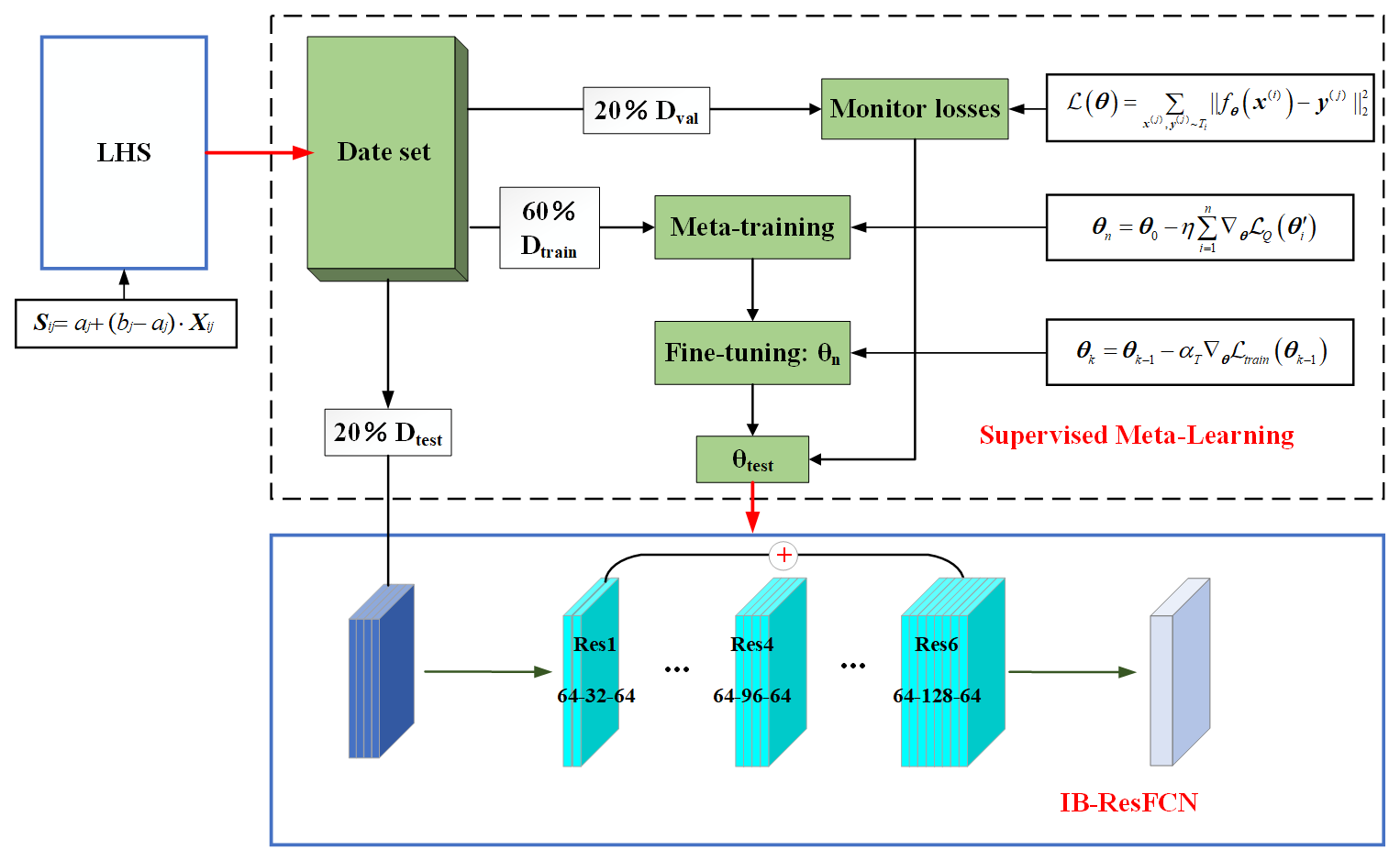
Figure 5 illustrates the overall workflow of meta-learning, primarily divided into the training phase and the evaluation phase: (1) first, establish the dataset using LHS; (2) separate the dataset based on distinct functional purposes; (3) start training the IB-ResFCN to obtain θ_test; and (4) assign the learned θ_test to the IB-ResFCN and evaluate it based on the test set.

3 Development of a parametric assisted design platform

Dataset construction requires modelling and finite-element analysis (FEA) for each sample. Sequential manual modelling for different samples entails a significant workload and low efficiency. Currently, parametric modelling is widely adopted, effectively reducing the time required to generate models. However, existing research rarely couples parametric modelling with FEA software for rapid modelling and analysis. This study develops an integrated platform coupling parametric modelling with FEA, significantly enhancing the efficiency of dataset construction.

The platform was developed within the Visual Studio development environment. Through API integration, the platform achieves direct invocation and collaborative control of SolidWorks and Abaqus, demonstrating robust system integration capabilities and cross-platform compatibility. The platform's overall architecture follows a “three-tier coupling, closed-loop-driven” technical approach. It comprises three core functional modules: the interaction layer, the logic layer, and the execution layer. The platform seamlessly integrates user input, data processing, and simulation computation, forming a complete closed-loop design–simulation cycle.

The interaction layer serves as the human–machine interface of the platform, implementing a graphical interface based on C# and WinForm technology. Users can intuitively perform parameter configuration and process control. As illustrated in Fig. 6, the overall interface consists of a parameter input zone, a structure preview zone, and a data management zone. The parameter input zone includes 25 critical fundamental parameters such as ball radius, guide rail dimensions, and mesh size. The structural schematic is embedded centrally, displaying key geometric features and dimension annotations. The data management zone enables custom file path configuration, automated saving strategies, and systematic organization of simulation results.

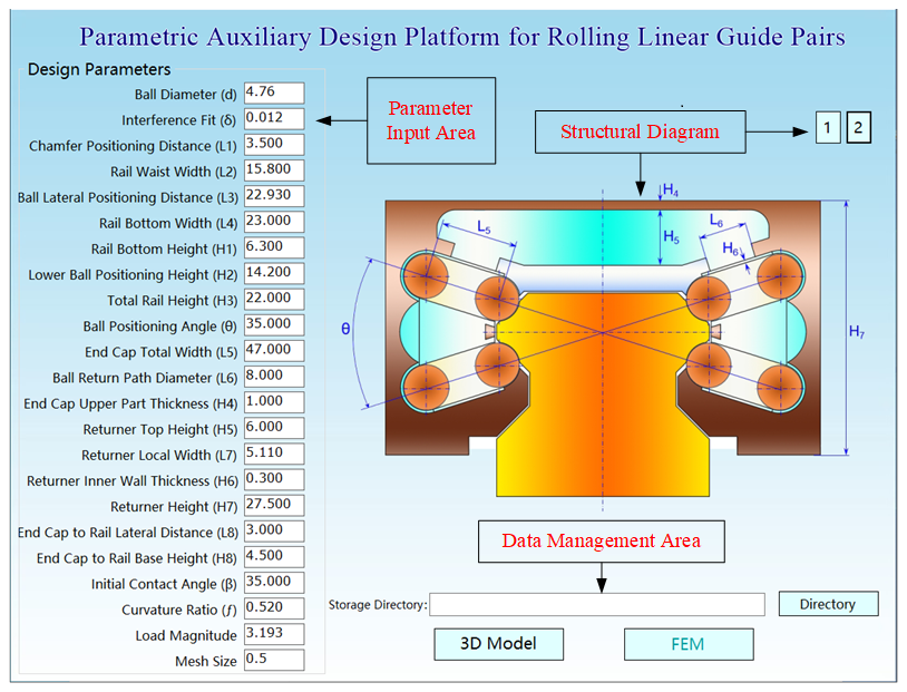
Figure 6 Schematic diagram of the parametric-platform interface. Dimensions in mm, loads in MPa, and mesh units in mm². The structural schematic references Structural Diagram 2 as an example.

Building upon parameter acquisition in the interaction layer, the logic layer acts as an intermediary bridge. It maps fundamental user inputs (e.g. ball diameter d, ball-positioning angle θ, initial contact angle β) into structural feature quantities required for modelling (guide rail dimensions, ball positions, assembly relationships, etc.). This mapping relationship can be mathematically formulated as follows:

$$\begin{array}{}\text{(13)}& \mathit{S}=f\left(\mathit{P}\right),\end{array}$$

where P= (d, θ, β,...) denotes the input parameter set; S represents the structural feature set required for modelling; and the mapping function f (⋅) is implemented through function fitting, lookup tables, or polynomial interpolation. To more clearly demonstrate the mapping relationship between S and P, the linear guide shown in Fig. 7 is taken as an example, with Table 3 providing specific mappings of key parameters. Through the mapping mechanism in the logic layer, automated modelling of structural-logic construction algorithms driven by dimensional chains is achieved.

Figure 7 Parameters for parametric modelling of the linear guide.

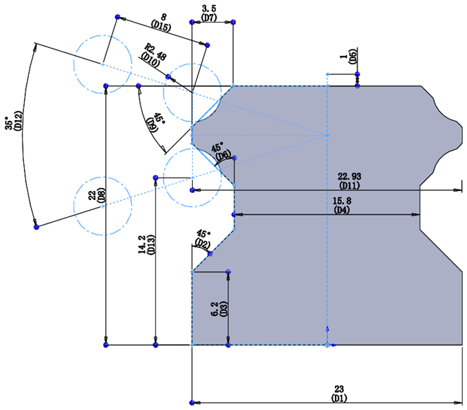
Table 3 Mapping relationship between S and P for the linear guide.

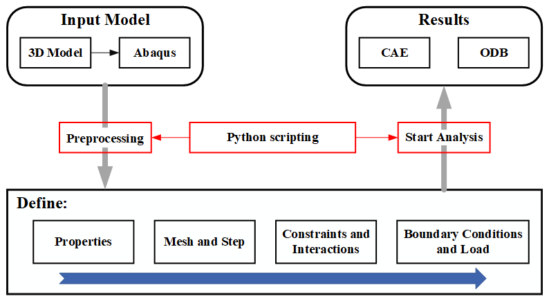
The execution layer covers two core processes: 3D modelling and FEA. Upon model completion, we select the FEM option in Fig. 6 to initiate FEA. As shown in Fig. 8, the STEP file exported from SolidWorks retains complete assembly information of the guide rail mechanism. Upon reading the file, the platform automatically imports the model into Abaqus. Subsequently, the pre-configured Python script file (py.) is automatically retrieved. This file contains command streams for preprocessing tasks and job submission modules. The platform automatically controls Abaqus to execute the complete workflow, including defining properties, meshing, setting boundary conditions, and so on.

Figure 8 Automated FEA workflow diagram.

Upon completion of the solving process, the platform automatically archives both CAE simulation files and ODB result files. This integrated system achieves rapid modelling and automated FEA, substantially enhancing the efficiency of dataset construction. As shown in Table 4, an experiment was conducted to evaluate the efficiency and reliability of the parametric platform. This study compared the traditional design method with the parametric-platform design method.

Table 4 Performance comparison between traditional design and parametric platform.

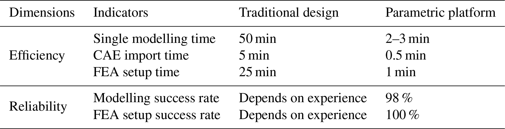
Initially, 100 sets of guide samples were randomly generated for modelling and simulation on the platform. Subsequently, 10 sets of models were randomly selected from the 100 sets of 3D models for manual modelling. The results indicate that, although a very small number of models failed due to parameter interference, the modelling success rate reached 98 %. With high reliability, the platform boosts single-iteration efficiency dozens of times over traditional methods.

4 Result analysis

4.1 Validation of FEA results vs. experimental results

In FEA, many components of the guide rail are non-load-bearing; it is thus necessary to simplify the overall model. The rolling linear guide pair is divided into several independent structural units, with each representing a repetitive structure of the guide assembly. Each unit includes three parts: the guide rail block, the slider block, and the upper- and lower-ball sets.

In the preprocessing module, the elastic modulus and Poisson's ratio for the ball–groove contact are set to $E=\mathrm{2.06}\times {\mathrm{10}}^{\mathrm{5}}$ MPa ν=0.3. For mesh generation, the multi-zone partitioning method is employed to obtain hexahedral meshes, with mesh refinement being applied to the contact regions. Surface-to-surface contact is adopted to ensure proper interaction at the ball–groove interface. A load is applied to the top of the slider, while full constraints are imposed on the bottom of the guide rail.

Vertical stiffness is a critical metric for assessing guide rail pair performance. It quantifies vertical deformation under vertical loads, defined by the following:

$$\begin{array}{}\text{(14)}& K_{\mathrm{v}}={\displaystyle \frac{P}{\mathrm{\Delta }{h}_{\mathrm{v}}}},\end{array}$$

where P denotes the external load, K_v represents the approximate vertical stiffness, and Δh_v indicates the deformation magnitude in the vertical direction. For the FEM of an independent structural unit, the schematic diagram of its simulation model is shown in Fig. 9, with the load distribution given by $P_{\mathrm{0}}=P/n$. β denotes the contact angle, defined by the oblique line connecting the curvature centres of the guide groove, the ball, and the slider. Since the groove radii of the guide rail and slider are identical, their vertical deformations are approximately equal. The total vertical deformation is given by $\mathrm{\Delta }{h}_{\mathrm{v}}=\mathrm{\Delta }{h}_{\mathrm{1}}+\mathrm{\Delta }{h}_{\mathrm{2}}$.

Figure 9 Schematic diagram of the simulation model.

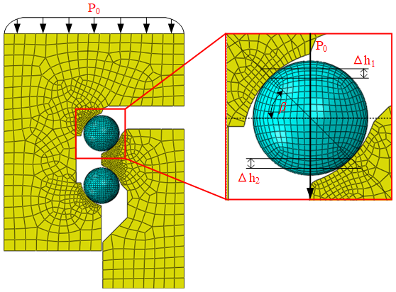
Through this method, the vertical deformation of the guide rail pair can be obtained. Substituting this value into Eq. (14) yields the vertical stiffness. However, inherent errors in FEA preclude achieving exact vertical-stiffness values, yielding only approximate results. To verify the accuracy of FEA results. This study takes the D45 guide pair as the subject, conducting static experiments to compare the Δh_v from FEA.

The full-parameter test bench for rolling linear guide pairs is illustrated in Fig. 10, primarily composed of a measurement system and a control system, a hydraulic system, and a mechanical system. Figure 10b displays the mechanical system comprising both loading and measurement components. The measurement components primarily include a contact displacement sensor (linearity error ≤0.5 % F.S), an S-shaped tension–compression load cell (linearity error ≤0.5 % F.S), signal amplifiers, and communication modules. The contact displacement sensor converts internal movement caused by operational accuracy variations into electrical signals. These signals are then transmitted to the control system via an amplifier, a communication module, and RS232 serial communication. The S-shaped tension–compression load cell generates resistance signals in response to external force variations, which are converted into digital communication signals by a signal amplifier and then are transmitted to the control system via RS232 serial communication. Once the signals enter the control system, the acquisition program collects, displays, and saves them.

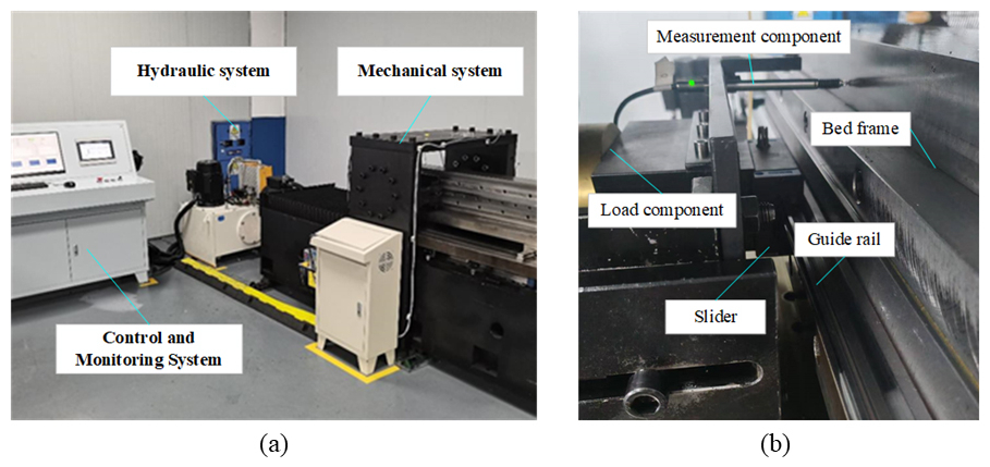
Figure 10 Full-parameter test bench for rolling linear guide pairs. Panel (a) shows the test bench, and panel (b) shows the mechanical system.

The testing procedure is as follows: install the rolling linear guide on the test bench. Apply load through the hydraulic system, increasing stepwise from 0 to 20 kN in 5 kN increments. First, obtain the force and displacement vectors at each node under the initial load condition. Next, calculate the variation in force and displacement at each measurement point. This variation is relative to the initial load condition during each force-holding period. After averaging the data, the resulting values represent the force and displacement for that time period. Finally, apply the least squares method to fit the force–displacement curves across all time periods, thereby deriving the vertical displacement.

Figure 11 Comparative results of experimental data and FEM.

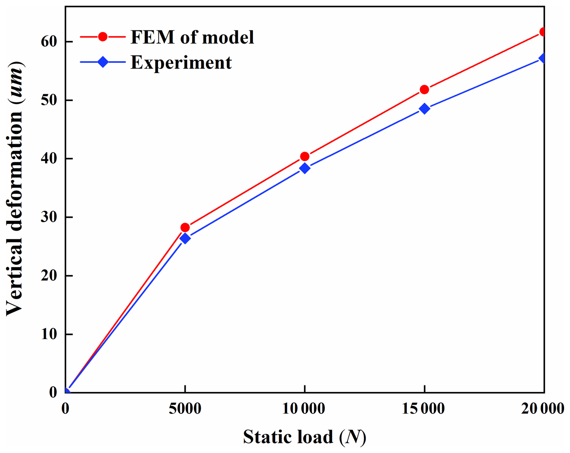
The obtained experimental results are compared with FEM, with the comparative outcomes being illustrated in Fig. 11. To quantitatively evaluate the prediction accuracy of the finite-element model, multiple statistical error metrics were calculated based on the aforementioned data, as shown in Table 5.

Table 5 Statistical errors of finite-element model predictions.

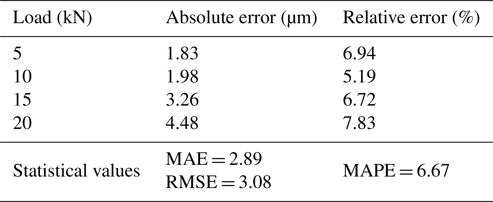
Results demonstrate a high degree of consistency between FEA and experimental outcomes, confirming the accuracy and validity of the finite-element model. This validated model can be reliably utilized for subsequent research tasks.

4.2 Influence of structural parameters on mechanical performance

Using the finite-element model in Fig. 8, we analyse the influence of different parameters on the mechanical performance of the guide rail pair. The parameters and their value ranges are as follows:

1. initial contact angle β (30–60°) – complementary angle of the load direction relative to the raceway-transmitted resultant force on rolling elements;

2. curvature ratio f (0.5–0.6) – the ratio of the groove radius of the guide pair to the ball diameter;

3. ball-positioning angle θ (27–37°) – angle between the upper-left/lower-right raceway centre line and the lower-left/upper-right raceway centre line;

4. interference fit δ (5–50 µm) – the value of interference between the balls and the grooves of the guide rail and slider.

Taking vertical deformation as the research object, FEA is conducted under loads of 5–20 kN, with β, f, θ, and δ as single variables. The influence of contact parameters on the vertical deformation of guide rail pairs is demonstrated, as detailed in Fig. 12.

Figure 12 Influence patterns of contact parameters on guide rail pairs.

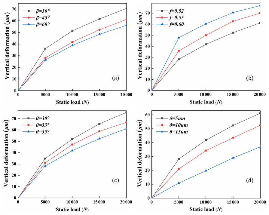
Analysis reveals that variations in contact parameters profoundly alter the mechanical performance of rolling linear guide pairs. Furthermore, this study systematically quantified the degree of influence of various parameters on the Δh_v of the guide pair. As shown in Fig. 13, the samples were collected based on LHS. The multi-factor global sensitivity analysis method (Lamboni and Kucherenko, 2021) was employed, systematically analysing the main effects and total effects of each parameter.

Figure 13 Multi-factor global sensitivity analysis.

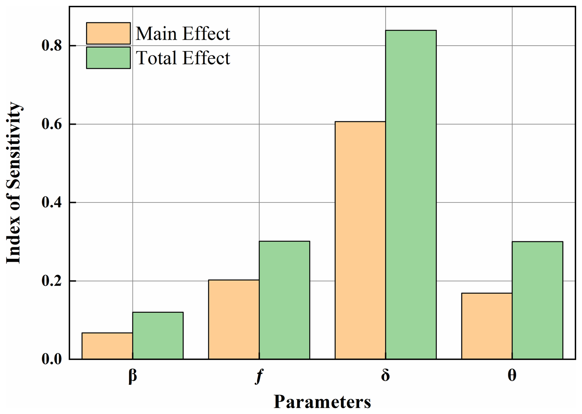
The results indicate that the interference fit is the dominant parameter affecting vertical displacement (0.839). The ball-positioning angle and curvature ratio also exert moderate influences, while the contact angle demonstrates a minimal effect (<0.1). Furthermore, the total effects of all four parameters consistently exceed their respective main effects. This finding reveals significant interaction effects among the parameters, where their synergistic interplay collectively governs the vertical displacement. Therefore, the geometric parameters of the contact zone can serve as inputs, with vertical deformation and maximum contact stress as outputs. A neural network with four inputs and one output is constructed as shown in Fig. 14. This network is trained to predict mechanical performance.

Figure 14 Neural network inputs and outputs for parameter optimization.

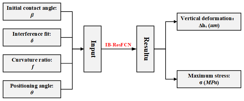
The prediction models for vertical deformation and contact stress share identical architectures, differing only in terms of parameters such as sample sets, data partitioning, and meta-learning rates.

4.3 Comparative analysis of network models

This section validates the structural rationality of the IB-ResFCN model and its prediction accuracy. Comparative validation experiments involving multiple models were conducted.

Taking the vertical deformation prediction model as an example, comparative experiments were designed for three key aspects: models with and without meta-learning, with and without inverted-bottleneck structures, and with and without residual connections. Experiments compared the proposed model against a conventional FCNN. Mean absolute error (MAE), root mean square error (RMSE), and coefficient of determination (R²) serve as evaluation metrics.

Figure 15 presents the results of comparative experiments. To ensure statistical reliability, this study adopts the 5-fold cross-validation method. The complete dataset was randomly partitioned into five similarly sized subsets, with each subset sequentially serving as the test set for performance evaluation to avoid chance results arising from specific data partitioning. Table 6 presents the statistical results of the 5-fold cross-validation, including the mean values of three metrics for each model. Furthermore, based on the 5-fold cross-validation results, the 95 % confidence intervals for each metric were calculated using the t distribution (with t=4).

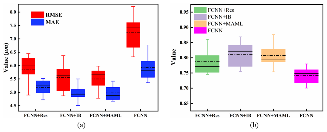
Figure 15 Comparative experiments. The black lines in both subfigures indicate median values, while the dotted lines represent mean values. Subfigure (a) displays the RMSE and MAE values for each model, and subfigure (b) shows their corresponding R² values.

Table 6 The 5-fold cross-validation performance metric statistics.

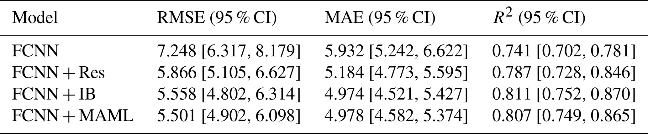
Overall, the improved models show significant advantages over traditional FCNN in terms of both accuracy and stability. In terms of prediction accuracy, the FCNN + IB model achieved the highest coefficient of R² among all compared models. Regarding stability, the FCNN + MAML model demonstrates optimal performance in error control, achieving the lowest values in terms of RMSE. Statistically, all improved models show superior performance compared to the baseline model, with their 95 % CIs showing minimal overlap or complete separation. This demonstrates the effectiveness of the model improvements, their statistical significance, and the strong robustness across different data partitions.

Furthermore, this study conducted ablation experiments to investigate the impact of dimensional design in the IB-ResFCN. Based on the network framework structure described in Sect. 2.2, a systematic comparison was conducted of the model's predictive performance across different dimensions.

As shown in Table 7, dimensional variations directly impact the model's final prediction accuracy. Based on the comparison of three accuracy metrics, the dimensionality (64–32/48/64–64) was determined to be the optimal configuration. This outcome is the prediction result for the vertical deformation model. Figure 16 presents the prediction results of both the vertical deformation and contact stress models.

Table 7 Comparison of ablation experiment data.

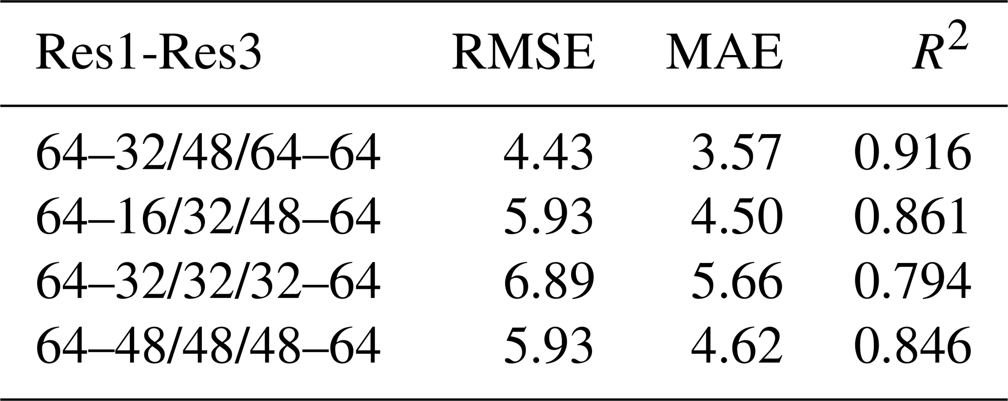
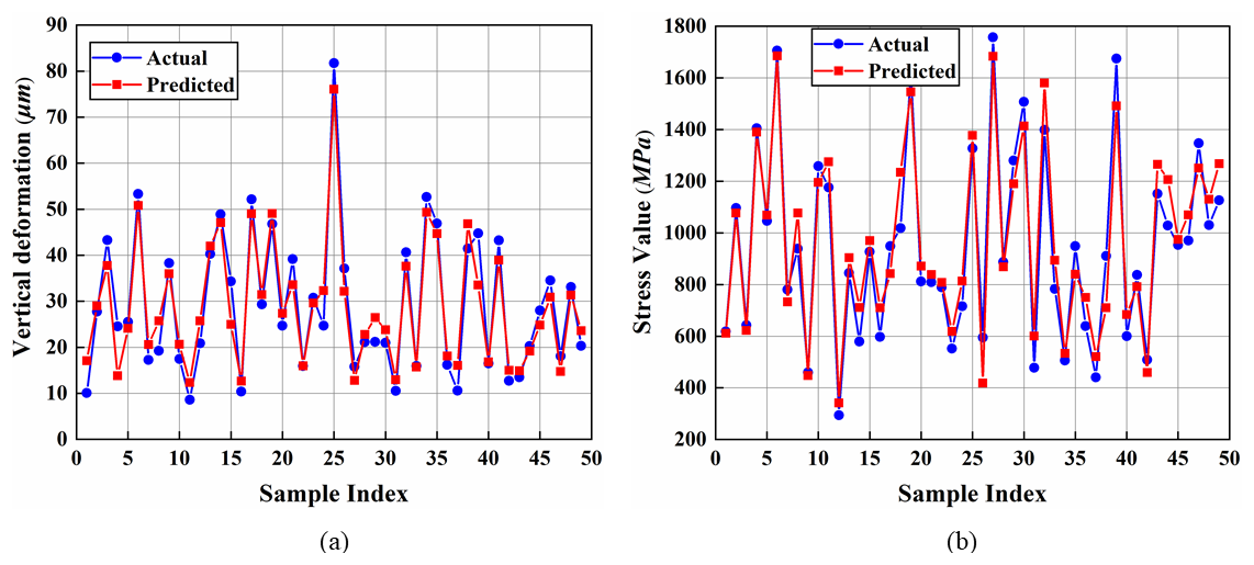
Figure 16 Prediction results. The stress prediction model accuracy metrics are as follows: MAE = 83.42, RMSE = 99.23, and R² = 0.924.

Figure 17 Loss curve during meta-training.

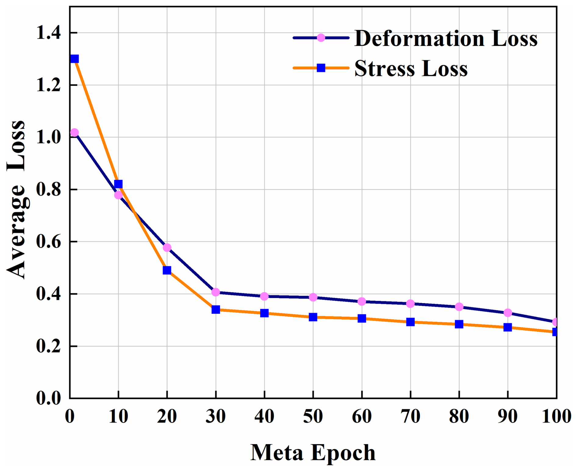
Furthermore, Fig. 17 illustrates the loss evolution curve during the meta-training phase. After approximately 30 training cycles, the meta-training loss reached a plateau. This phenomenon is related to the designed distribution of meta-tasks: during each meta-iteration, the model processes a batch containing N=20 distinct tasks, where each task is constructed by randomly sampling K=15 data points from the training set. These are divided into support sets (10 samples) and query sets (5 samples) for meta-gradient computation. This random sampling strategy ensures the diversity and representativeness of training tasks. The initial rapid decline in loss stems from the model learning a robust set of initialization parameters. The observed plateau suggests successful learning of the underlying task distribution patterns. Additional meta-training iterations provide negligible improvements. With the loss value stabilizing, the model exhibits rapid adaptation ability for tasks from comparable distributions.

4.4 Optimization solving results

The sensitivity analysis in Sect. 4.2 demonstrates how structural parameters affect vertical stiffness. These parameters interact in complex ways and not through simple linear addition. To address this challenge, the SLSQP algorithm from SciPy's optimization library was implemented. This method (Gill et al., 2005) proves to be highly effective for constrained optimization problems characterized by smooth nonlinear functions in both objective and constraint formulations.

4.4.1 Constraint conditions and convergence criteria

The SLSQP algorithm transforms nonlinear constrained problems into sequential quadratic programming subproblems. This iterative approach efficiently converges to optimal solutions. This approach integrates two classical optimization algorithms: sequential quadratic programming (SQP) and least squares (LS). This algorithm proves to be effective for solving the constrained optimization problem in this study:

$$\begin{array}{}\text{(15)}& \begin{array}{rl}& \begin{array}{c}\text{minimize}\\ x\in R^{\mathrm{4}}\end{array}\mathrm{\Delta }{h}_{\mathrm{v}}\left(\mathit{x}\right)\\ & \mathrm{subject}\mathrm{to}g\left(\mathit{x}\right)\left[\mathit{\sigma }\right]-{\mathit{\sigma }}_{\max }\left(\mathit{x}\right)\ge \mathrm{0}\\ & {\mathit{x}}^{\mathrm{l}}\le \mathit{x}\le {\mathit{x}}^{\mathrm{u}},{\mathit{x}}^{\mathrm{l}}=\left[{\displaystyle \frac{\mathit{\pi }}{\mathrm{6}}},\mathrm{5},{\displaystyle \frac{\mathrm{1}}{\mathrm{2}}}{\displaystyle \frac{\mathrm{27}\mathit{\pi }}{\mathrm{180}}}\right],{\mathit{x}}^{\mathrm{u}}=\left[{\displaystyle \frac{\mathit{\pi }}{\mathrm{3}}},\mathrm{50},{\displaystyle \frac{\mathrm{3}}{\mathrm{5}}}{\displaystyle \frac{\mathrm{37}\mathit{\pi }}{\mathrm{180}}}\right],\end{array}\end{array}$$

where the optimization variable x∈R⁴ represents the structural parameters from Sect. 4.2; Δh_v(x) is the minimization objective function; g(x) denotes the constraint function; and “l” and “u” respectively define the lower and upper bounds of the optimization variables. Within the constraint conditions, the maximum allowable stress is [σ]=800 MPa, and σ_max(x) represents the predicted maximum stress value.

The SLSQP algorithm handles these constraints through an internal Lagrangian formulation. This formulation consistently maintains solution feasibility throughout the optimization process rather than employing an external penalty method. The convergence criteria are specified as follows:

1. function value tolerance – ftol = $\mathrm{1}\times {\mathrm{10}}^{-\mathrm{6}}$ (relative change in objective function);

2. parameter step tolerance – xtol = $\mathrm{1}\times {\mathrm{10}}^{-\mathrm{6}}$ (maximum change in optimization variables);

3. maximum iterations – 300 (computational budget limit).

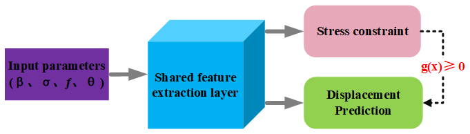
These complementary tolerances ensure convergence stability. The optimization process terminates when any condition is met. This approach ensures both computational efficiency and high-quality solutions. Figure 18 illustrates the dual-network framework implementing this algorithm.

Figure 18 Schematic of dual-network joint architecture.

4.4.2 Multi-start optimization results and sensitivity analysis

To ensure optimization reliability and to mitigate local optima risks, this study implements a comprehensive multi-start strategy. Starting from 100 randomly generated initial points within the feasible region, the SLSQP algorithm was executed independently for each starting configuration. Figure 19 displays the distribution histogram of vertical deformation values obtained from 100 optimization runs.

Figure 19 Distribution histogram of vertical deformation values.

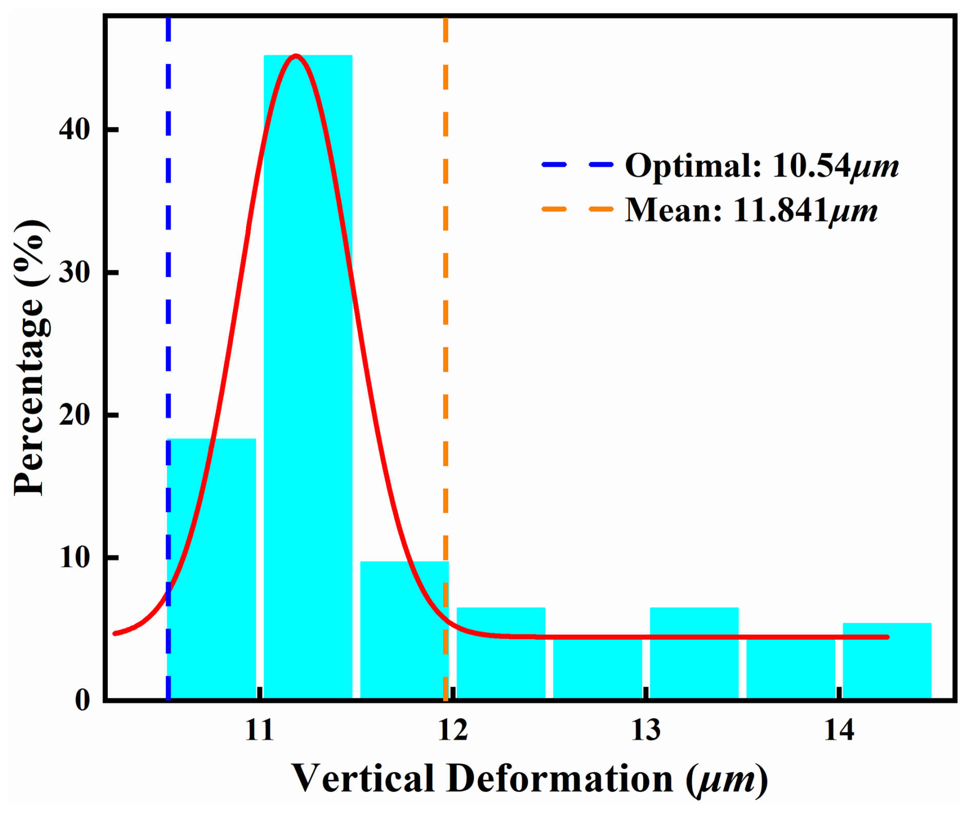
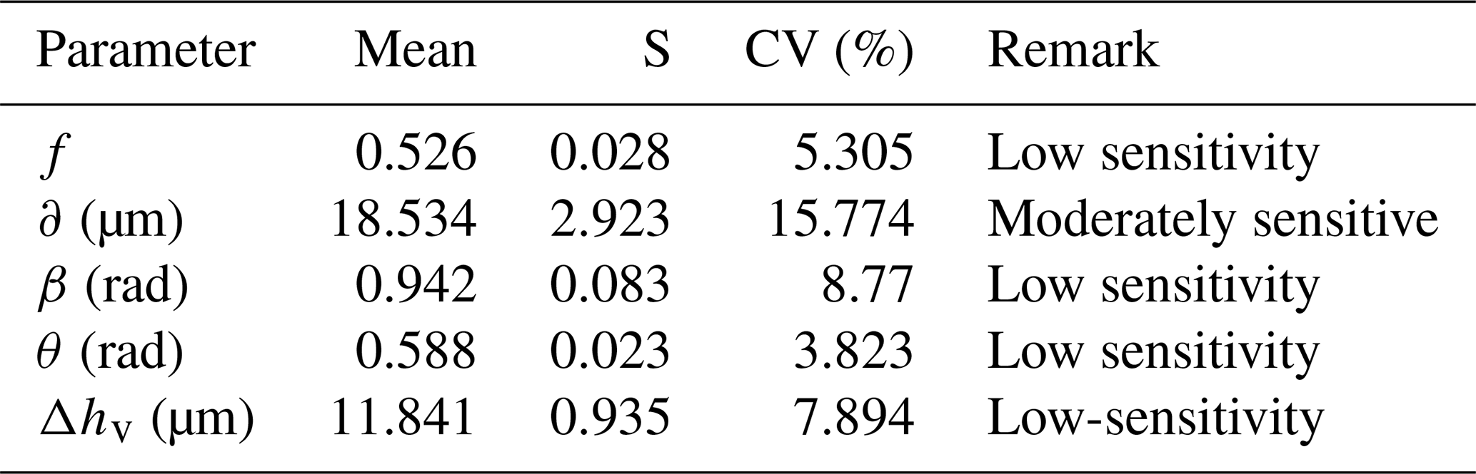
Results indicate an optimization interval of [10.54, 14.50], and the success rate is 94 %. Over 70 % of results exceed the mean value, clustering tightly near the optimum. The optimal solution is reachable from diverse initial conditions. These results further confirm the stability of the optimization algorithm. Additionally, this study conducted a sensitivity analysis of the initial conditions. As shown in Table 8, we calculate the coefficient of variation (CV) for all optimal parameters. The Δh_v, β, f, and θ all exhibit CV values below 10 %. These are classified as low-sensitivity parameters. The δ demonstrates a CV value between 10 %–20 %, classifying it as moderately sensitive. This necessitates strict tolerance control during actual manufacturing.

Table 8 Sensitivity analysis of optimized parameters.

For clearer demonstration of performance metric trade-offs across the design space, Fig. 20 shows the distribution of all feasible solutions within the design space. In the figure, the red line indicates the stress constraint, while the magenta line represents the overall variation trend. The results show a positive correlation between vertical deformation and maximum contact stress. This trend indicates that, under the stress constraint condition, pursuing high stiffness typically requires reducing contact stress. Therefore, optimizing structural parameters improves these two critical performance metrics concurrently.

Figure 20 Distribution of feasible solutions in the performance space.

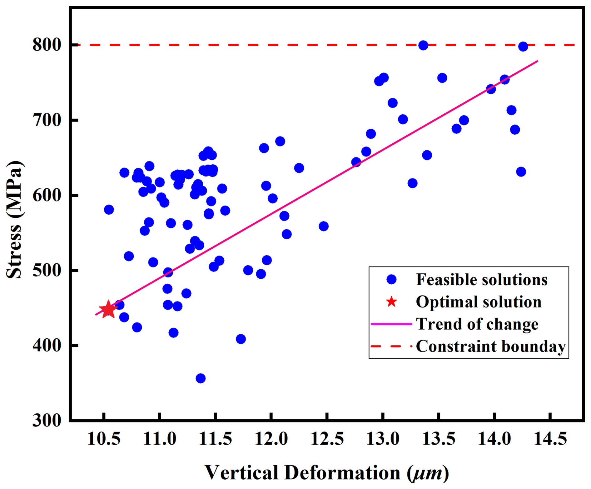
Table 9 demonstrates that the optimized guide rail pair achieves a 57 % reduction in vertical deformation, a significant enhancement in vertical stiffness, and a declining trend in maximum stress values.

Table 9 Initial parameters vs. optimized parameters.

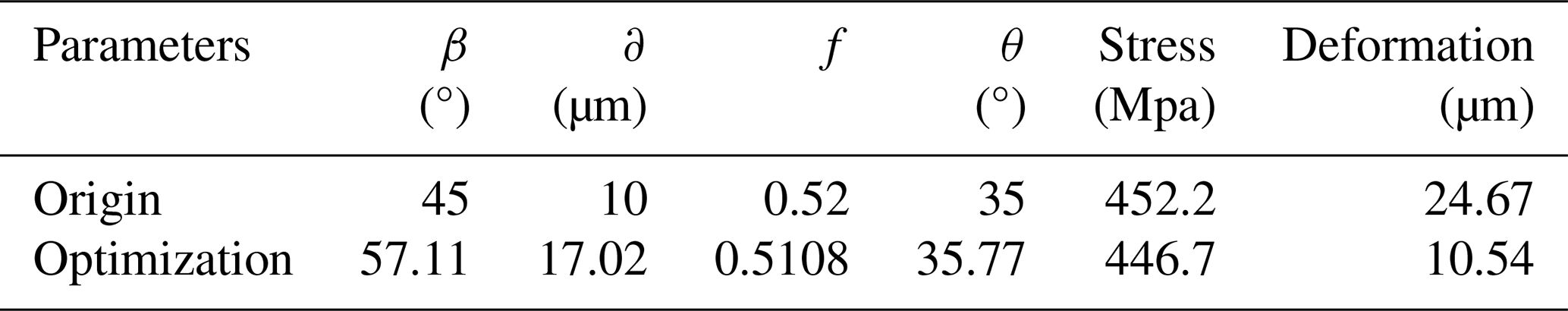
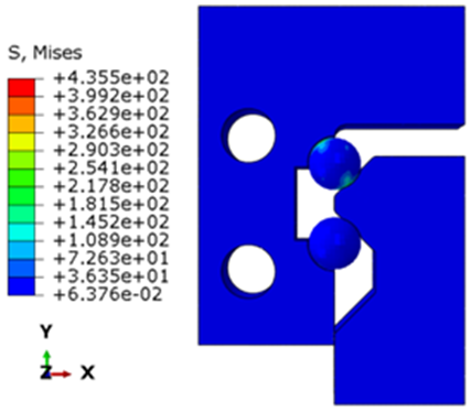
To ensure the accuracy of optimization results, the optimized parameters are input into a parametric platform for modelling and simulation validation, with the outcomes illustrated in Fig. 21. Validation shows a mere 2.9 % deviation in maximum stress values and only 9.7 % variation in extracted vertical deformation. Consequently, the optimization results demonstrate high accuracy.

Figure 21 Finite-element validation diagram.

Compared with traditional FEA optimization methods, this study develops a workflow encompassing neural network modelling, dual-network collaborative frameworks, and optimization solving to derive an optimal set of structural parameters.

5 Conclusions

This study addresses the multi-objective optimization design problem for rolling linear guide rail pairs. An intelligent optimization framework based on a meta-learning surrogate model is proposed in this study. This method significantly relieves the over-reliance on costly FEM in traditional design processes and effectively addresses the challenge of constructing high-precision models with limited sample data. This study conducts the following research:

1. A platform integrating parametric modelling and automated FEA was developed. This approach dramatically enhances the efficiency of sample data generation, providing a highly reliable dataset for surrogate models.

2. An IB-ResFCN model was constructed by integrating the inverted-bottleneck residual structure with FCNN. Through a MAML training strategy, the model achieves over 90 % prediction accuracy for mechanical performance under few-shot conditions.

3. Based on the constructed surrogate model, the SLSQP algorithm is employed for multi-objective optimization of key structural parameters. Results demonstrate that the optimized structure achieves significantly enhanced mechanical performance, fully validating the effectiveness and engineering value of the proposed optimization method.