the Creative Commons Attribution 4.0 License.
the Creative Commons Attribution 4.0 License.
 | 17 Nov 2026
Tolerance-forward-mapping-based multi-body system kinematic error prediction model for five-axis machine tools
Hongxia Yan

Wenliang Luo
Yupeng Zhao
Improved accuracy of five-axis machines is vital, and one way to achieve this is by optimizing tolerances for important components. It is well known that there are no quantitative models based on which design tolerances can directly be correlated with machining errors. The result is often trial-and-error and manual adjustments. It is therefore hard to predict and control accuracy. To address this problem, the authors propose a tolerance-forward-mapping-based multi-body system (MBS) kinematic error prediction model (TFM-MBS) and test its effectiveness experimentally. First, a Fourier series superposition is used to map the tolerance parameters of the key parts with geometric errors. The periodicity of the errors is reflected in the data; using MBS and homogeneous transformation matrix (HTM) integration of the geometric error volumetric model and an ideal S-shaped path, a complete error prediction model is proposed. Experiments were performed under one cutting condition, and predicted and measured errors were obtained in the workpiece's four sections. The average predicted contour error in these sections was 0.0450, 0.0448, 0.0446, and 0.0455 mm, respectively, while the measured contour error was 0.0475, 0.0472, 0.0474, and 0.0477 mm. All deviations were within 6 % of the preliminary verification of the model in geometric-error-dominated conditions. The model provides a theoretical basis for quantitative optimization of machine-tool tolerance design but does not take into account nonlinear factors such as thermal deformation, vibration, of force-induced deformation.
- Article
(5474 KB) - Full-text XML
- BibTeX
- EndNote


A high-precision five-axis machine is a key technology for aerospace structural components where form tolerances are often lower than 20 µm. As aerospace, biomedical, and electric-vehicle propulsion systems demand increasingly stringent form tolerances, geometric errors have become the main bottleneck limiting machining efficiency, dimensional accuracy, and long-term service reliability (Ding et al., 2023; Yang et al., 2025). More refinements in assembly and fabrication can mitigate such errors, but elimination is economically impossible (Zhang et al., 2024). Designers must reconcile residual deviations with tight quality specifications, which increasingly requires rational tolerance regimes grounded in systematic optimization rather than intuition.
The conventional sequential design, where parameter selection precedes tolerance specification, suffers from inherent inefficiency: tolerance grades determined at the second stage often render initial parametric choice suboptimal and require repeated rework (Lv et al., 2023). Since the tolerance assignment is based on heuristic trial-and-error and empirical rules, it is rarely informed by quantitative tradeoff analyses (Duan et al., 2024; Armillotta, 2024). Optional systems exist such as the genetic algorithm proposed by Thilak et al. (2023) for tolerance chain identification, which implicitly assumes linear independence among tolerances. This is broken for multi-axis machines where geometric errors are coupled kinematically across the structural loop. Such coupling implies tolerance effects can be treated additively. No current method provides system-level mapping from component tolerances to final errors before hardware build.
Geometric error modeling has long been a cornerstone of precision analysis, yet its role remains predominantly diagnostic – quantifying errors in existing machines – rather than prescriptive – guiding tolerance decisions prior to manufacture. Extensive studies have refined measurement techniques, compensation algorithms, and volumetric error models for both linear and rotary axes (Wang et al., 2021; Sun et al., 2023; Fan et al., 2024; Lv et al., 2025; Zhang et al., 2025a; Wu et al., 2022; Ye et al., 2026).
Despite these advances, the vast majority of existing models serve post hoc compensation – an orientation extensively reviewed by Schwenke et al. (2008) and reflected in a variety of measurement methodologies (Chen et al., 2001). They accept given geometric errors as inputs and compute volumetric deviations, but they cannot invert the relationship to determine which tolerance specifications yield acceptable errors at minimum cost. Thermal distortion further complicates the problem, but even advanced thermo-geometric compensation is not enough to bridge design–diagnosis dichotomy (Niu et al., 2025; Liu et al., 2025).
Instrument-based error detection (although very complex) is still diagnostic and expensive, mostly restricted to R&D laboratories (see recent work on rotary-axis error identification by Peng et al. (2024) and on-machine sensor calibration by Wang et al., 2024). A better alternative is to shift verification burden from physical measurement to virtual prediction. If tolerance design can establish mapping from design tolerances to final machining accuracy, designers can screen candidates before hardware is built, thus reducing trial cuts and coordinate measuring machine (CMM) inspections.
The S-shaped test piece, formally incorporated into ISO 10791:2020 (Part 7), exemplifies this paradigm: it serves not merely as a diagnostic artifact but as a calibration target for tolerance–error prediction models, with proven discriminative power in complex-surface machining (Osei et al., 2023).
The current state of the art thus exhibits two gaps: (i) no systematic mapping from tolerances to final errors and (ii) over-reliance on empirical heuristics. The present paper addresses these gaps by introducing Fourier-based tolerance–error mapping, Sobol-index-based global sensitivity analysis (GSA), and validation on the S-shaped specimen.
The proposed framework unfolds in three sequential tiers. Tier 1: forward propagation establishes a Fourier mapping. A volumetric error model using MBS and HTM is used to predict spatial contour errors directly from tolerance inputs. Tier 2: diagnostic prioritization is performed by Sobol index GSA in the predicted error space. This allows designers to define critical tolerances affecting variance in contour error. Designers can adjust tolerances to tighten the tolerances in critical areas, relax them in less critical areas, and retain quality. Tier 3: experimental validation of the whole framework is performed using an S-shaped test specimen under finishing. Comparisons are made between predicted contour errors at four cross sections and CMM measurements. These results show that the mapper predicts machining errors within acceptable engineering limits. This makes the mapper a useful prescriptive design tool and can be used for a paradigm shift from intuition-based trial-and-error tolerance assignments. It is hypothesized that periodic signatures of manufacturing-induced surface errors in key machine components can be represented in a Fourier series expansion with a clear truncation constraint based on physical conditions. It is suggested that propagation of the errors through the kinematic chain can be linearly superposed using MBS and HTM to predict final contour errors.
2.1 Modeling
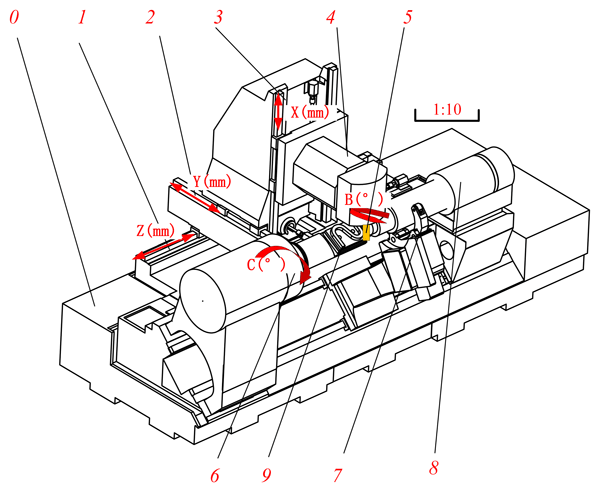
The five-axis machine schematic is shown in Fig. 1. There are three translational axes and two rotational axes, namely the X, Y, Z, B, and C motion axes. Linear errors are denoted by δ, with subscripts indicating the error direction and parentheses indicating the motion axis, totaling 15 items: δx(i), δy(i), δz(i), i=x, y, z, B, C. Rotational errors are denoted by ϵ, with subscripts indicating the direction of rotation about the axis and parentheses indicating the motion axis, totaling 15 items: ϵx(i), ϵy(i), ϵz(i), i=x, y, z, B, C. Squareness errors are denoted by ϵ, with subscripts indicating the two motion axes, totaling seven items: ϵxz, ϵyz, ϵxy, ϵxB, ϵBz, ϵxC, ϵyC, totaling 37 errors.

This diagram's key components are as follows: linear motion units and base, bed (0), and the Z axis (1), Y axis (2), and X axis (3) for achieving three linear motions; rotary motion units, the B axis (4) for tool oscillation, and the C axis (6) for workpiece rotation; machining system, tool (5), and the workpiece (9) to be machined; auxiliary supports, steady rest (7), and the tailstock (8) for stabilizing the workpiece.
2.2 Mapping relation
The prediction model for machining errors cannot be directly derived from tolerance parameters, as an unknown geometric error exists between them during the design phase. This geometric error is not merely an intermediate variable but rather a key medium that translates tolerance specifications into machining deviations. Quantifying tolerance–geometric error coupling is a prerequisite for precision design. Table 1 lists the definition and calibration of each tolerance.

The selection of Fourier series as the mathematical foundation for tolerance–error mapping is motivated by three physically grounded considerations. First, the finishing processes applied to guide rails, ballscrews, and spindle housings – namely precision grinding, milling, and lapping – imprint characteristic periodic signatures on the component surfaces. These signatures correspond directly to tool feed marks, grinding-wheel wear patterns, and spindle-rotation harmonics, all of which are periodic by nature. Second, the measured surface profiles of these precision-machined components satisfy the Dirichlet conditions (boundedness, piecewise continuity, and a finite number of extrema over the evaluation length), which guarantees the convergence of their Fourier expansions. Third, the Fourier basis provides a complete orthogonal set, offering both computational efficiency and physical interpretability: the first-order term captures the fundamental machining periodicity, while higher-order terms represent finer texture features.
Crucially, the retention of only the first-order Fourier term in the final mapping model is not an arbitrary choice made for mathematical convenience; rather, it emerges naturally from the wavelength-to-slide-length constraint introduced in this study. For a linear axis, the carriage (or slide) acts as a spatial moving-average filter over the guide-rail profile. Any Fourier component whose wavelength λ is shorter than the carriage length L produces no net angular or positional deviation over the full travel range, because the carriage integrates these short-wavelength undulations. Substituting the carriage length Lx=800 mm (see Table 2) into this constraint yields a cutoff wavelength of mm (). Since the dominant periodic errors from the manufacturing processes considered here have fundamental wavelengths well exceeding this threshold, only the first-order mode contributes significantly to the quasi-static geometric errors. This constraint provides a physical truncation criterion, avoiding the empirical order-selection problem commonly encountered in purely data-driven Fourier approaches.

It is acknowledged that a direct fast Fourier transform (FFT) analysis of the measured surface profiles was not performed in the present study – a limitation that is openly recognized. Nevertheless, the adopted Fourier representation remains a well-established and physically justified approach in surface metrology for characterizing periodic error components in precision machine-tool components. The wavelength-to-slide-length constraint further provides a deterministic basis for truncation, to avoid overfitting or arbitrarily selecting harmonics. Future work will incorporate experimental FFT identification to refine the harmonic coefficients of particular machines.
The moving parts of a five-axis machine are milled systematically as final step by introducing frequency-periodic ripples on the part surface. Wu et al. (2022) have demonstrated that for large structural components that satisfy Dirichlet boundary conditions, the surface shape error can be expanded into a Fourier series, with each harmonic component representing different scales of spatial frequency. Our research group previously established a mapping equation from tolerances to PDGEs (component geometric errors), where the perpendicularity error serves as a typical subset of PIGEs (quasi-static geometric errors), directly resulting from the numerical limitation of the perpendicularity tolerance. The correspondence between tolerances and PDGEs is shown in Fig. 2 (translational axes) and Fig. 3 (rotary axes). The definitions and specific values of the above parameters are shown in Table 2.


Machining tools typically include translational and rotational axes, whose geometric errors differ in nature and impact. The X axis and C axis exemplify these distinctions.
Tolerance definitions grouped by axis as follows.
-
X axis (t1–t4): t1: XOZ straightness; t2: XOY straightness; t3: positioning accuracy; t4: parallelism
-
Y axis (t5–t8): t5: YOZ straightness; t6: XOY straightness; t7: positioning accuracy; t8: parallelism
-
Z axis (t9–t12): t9: XOZ straightness; t10: YOZ straightness; t11: positioning accuracy; t12: parallelism
-
B axis (t13–t15): t13: angular positioning; t14: radial runout; t15: axial runout
-
C axis (t16–t18): t16: angular positioning; t17: radial runout; t18: axial runout
-
Perpendicularity (t19–t25): t19 through t25: perpendicularity tolerance
2.3 Spatial motion error model
Model assumptions and limitations
The model can be described by several assumptions that not only govern the modeling process but also have a significant influence on the results.
One of them is the linear superposition assumption. It assumes geometric error fields are linear superpositions, without any nonlinear coupling. This assumption is reasonable when the error magnitude is small, but it may introduce deviations in the case of large errors.
Rigid-body assumption: each component in the MBS is regarded as a rigid body, and elastic deformations are ignored. This assumption is applicable to static or quasi-static error analysis, but it cannot represent dynamic cutting effects.
Ignoring thermal errors: the modeling controls the measurement environment temperature but omits machine-tool thermal deformation. In actual processing, thermal drift may become the main error source.
Unmodeled dynamic effects of tools and spindles: dynamic effects such as tool deflection and spindle vibration are not included, and the model is suitable for low-speed or light-load processing conditions.
Periodic error assumption: the surface errors of the part are described using Fourier series, which is applicable to precision machining surfaces but has limited applicability for rough machining or non-periodic errors. The MBS was modeled per Fig. 4.

The machine tool comprises two independent kinematic chains, as illustrated in Fig. 4.
-
Tool chain: 0 (Bed) → 1 (Z axis) → 2 (Y axis) → 3 (X axis) → 4 (B axis) → 5 (Tool)
-
Workpiece chain: 0 (Bed) → 6 (C axis) → 7 (Steady rest) → 8 (Tailstock) → 9 (Workpiece)
Based on the MBS topological structure, 4×4 HTM are employed to describe the positional and orientational relationships between any adjacent bodies i and j.
{Qj}i: the position matrix of point Q in Oi−xiyizi; {rj}i: the position matrix of point Q in Oj−xjyjzj; : the nominal position matrix; : the actual position matrix; : the nominal motion matrix; : the actual motion matrix.
In the workpiece branch, the position vector of the tool center point (TCP) is
In the tool branch, the position vector of the TCP is
The two branch TCPs must coincide.
From Eqs. (14)–(16), the TCP position vector in the workpiece frame is
Expanding Eq. (17) (neglecting higher-order error terms) gives the actual TCP vector; with all error parameters zero, the nominal vector (workpiece frame, ideal) is
Finally, the volumetric error vector E at any arbitrary position within the machining space is defined as the vector difference between the actual tool position and the nominal tool position:
The components Ex, Ey, Ez are the positioning deviations in X, Y, Z and are directly used for contour-error compensation.
2.4 GSA
2.4.1 GSA for spatial errors
To investigate the comprehensive effect of tolerance values on errors at different spatial positions, this paper normalizes the spatial error model, as shown in Eq. (20).
The average processing spatial error is calculated according to Eqs. (19) and (20), as shown in Eq. (21).
The spatial error is a function of the error term t1, t2, t3, …, ti, as shown in Eq. (22).
The error function f(t) and analysis of variance formula can be expressed as follows (Eq. 23):
In Eq. (23), f0 is a constant. For the remaining decomposed subterms, when performing an integration operation on any of the independent variables within its domain, the integration result is zero, thus satisfying the orthogonality condition required for variance decomposition.
The subterms in Eq. (24) are orthogonal to each other, and the values of the subterms at each order can be expressed as f(t) integrals. The total variance in the output of the error function is shown in Eq. (25), and, simultaneously, Eq. (26) can be obtained as follows:
The influence of different tolerance parameters on spatial errors is analyzed using Eqs. (26) and (27). In Eq. (27), Si is the first-order sensitivity coefficient of the error term ti, which represents the degree of influence of the error term ti on the spatial error. Sij is the second-order sensitivity coefficient. When i and j are not simultaneously zero, it represents the combined influence of the two error terms ti and tj on the spatial error.
The overall sensitivity coefficient represents the sum of the first-order sensitivity coefficient of the error term ti and all higher-order sensitivity coefficients that have a joint effect with Si, as shown in Eq. (28).
2.4.2 Simulation calculation of GSA
The simulation calculation of GSA was executed in the MATLAB (R2022a) environment. The calculation results are shown in Fig. 5. Per axis (X/Y/Z) and global top-five sensitivity lists are
-
X {t9 (43.1 %), t17 (24.3 %), t10 (13 %), t12 (5.4 %), t16 (4.8 %)},
-
Y {t12 (48.6 %), t10 (20.1 %), t16 (13.7 %), t9 (7.2 %), t2 (5.3 %)},
-
Z {t17 (38.3 %), t1 (19 %), t4 (16.1 %), t8 (14.2 %), t11 (5.6 %)},
-
Overall {t12 (23.9 %), t17 (22.3 %), t10 (14.6 %), t1 (8.9 %), t4 (7.1 %)}.
Figure 6 shows that the Z axis angular deviation error (t12) and the C axis positional offset error (t17) are the most significant global tolerance sources affecting the overall spatial error of the machine, jointly accounting for over 46 % of the total error variance. In contrast, although the X axis straightness (t1) exhibits extremely high sensitivity in the Z direction (19.0 %), its overall contribution to the combined error is relatively limited at 6.9 %.


To validate contribution degree analysis, this paper selected critical tolerances 50 % smaller than original values and computed the spatial error (average spatial error is 28.9 to 20.4 µm, 29.4 % lower). In Fig. 7, the contribution degree of critical tolerances identified by sensitivity analysis is correct and provides a quantitative engineering basis for tolerances and accuracy allocation.

Milling experiments on S-shaped specimens were conducted to test the engineering feasibility of the model. The predicted contour errors were compared to actual measured errors.
3.1 Experimental setup
Cutting parameters based on ISO 10791 were used: moderate cutting conditions, 8000 rpm spindle speed, and a feed rate of 2000 mm min−1. The model is driven by geometry and kinematics. The aim is validation of the mapping relationship between tolerances, geometric error, and machining error. The authors chose a single stable cutting condition in order to avoid non-geometric physical factors such as cutting forces, vibrations, and thermal deformation. By selecting a stable cutting condition researcher ensured that the measured errors are mainly geometrical tolerances transmitted by essential machine components. This allowed the validation results to represent the kinematic model developed using MBS and HTM methods. This design choice has been clearly specified in the experimental methodology section.

The experimental specimens were made of 2A12 high-strength aluminum alloy, with overall dimensions of 310 mm × 210 mm and an S-shaped edge strip height of 30 mm. The parameters are shown in Table 3.
The positioning accuracy of its key axes is 8, 8, and 12 µm for the X/Y/Z axes, respectively. The B/C axis is 8 in. (20.32 cm). A ϕ10 mm TialN-coated carbide end mill was adopted. The cutting parameters were set as follows: spindle speed 8000 r min−1, feed rate 1200 mm min−1, and cutting depth 0.5 mm. Before processing, the machine tool should be preheated for no less than 30 min to enter a thermally stable state. The processing site is shown in Fig. 8.

3.2 Measurement and data acquisition
After processing was completed, the Zeiss CONTURA RDS7/10/6 CMM was used to collect the point cloud data on the surface of the specimen. The measurement repeatability of this equipment was 1.7 µm. Ambient temperature was controlled at 20 ± 0.5 °C to reduce thermal errors; see Fig. 9 for the site. The surface point cloud data of the processed specimens were collected using the Zeiss CONTURA RDS CMM in a temperature-controlled environment (20 ± 0.5 °C), with a measurement repeatability of 1.7 µm to ensure the high precision of the measured value of the contour error.

To comprehensively evaluate the predictive performance of the model under different geometric features, four feature detection sections (Z1–Z4) were selected along the edge height direction, and the section spacing is shown in Fig. 10. The heights of each cross-section from the base (Z0) are respectively Z1 = 10 mm (low-curvature zone), Z2 = 13 mm (transition zone), Z3 = 18 mm (high-curvature zone), and Z4 = 23 mm (free-edge zone), and the cross-sectional spacings are respectively Z1→Z2: 3 mm, Z2→Z3: 5 mm, and Z3→Z4: 5 mm. From each cross-section, 37 equidistant detection points were collected by CMM, and the measured value of the average contour error in this cross-section was calculated.

The four measurement sections are not equally spaced along the height direction, but instead correspond to four extreme and distinct tool kinematic characteristics during the machining of the S-shaped specimen.
-
Low-curvature region – quasi-static tool posture
-
Transition zone – sharp torsion of the tool axis vector
-
High-curvature regions – high-frequency abrupt changes in feed direction
-
Free-edge region – open boundary effect
Under these four typical kinematic conditions, the model's predicted profile deviation errors were consistently controlled within 6 % of the measured values, indicating that the mapping chain exhibits good robustness under complex multi-axis motions.
4.1 Calculation of contour error
Spatial error is derived from point-wise calculations within the working space, independent of part contour. To validate the error prediction model, this paper focus on the S-sample profile.

The workpiece's trajectory is shown in Fig. 11. The initial coordinates of the ideal path (0, 97.5, −57) are 0, −97.5, and −57, and the actual path (0.0003, −97.5423, −57.0037) is based on geometric errors due to tolerances of the parts (guide rail straightness variation, lead screw position, etc.). These tolerance-induced geometric errors generate micron-level offsets (maximum 0.0423 mm) along the machining trajectory, representing the primary source of subsequent workpiece contour errors.

Figure 12The figure shows the profile errors in the ideal and actually obtained S-shaped test specimens at Z1, Z2, Z3, and Z4.
When the workpiece rotates with axial feed, the swing head generates a helical path on the surface, from which the S-sample profile is derived. As shown in Fig. 12, setting the tool height and workpiece rotation yields both ideal and actual simulation curves.
The measured average contour errors for sections Z1–Z4 were all approximately 0.047 mm, with the Z4 section exhibiting the highest value and Z2 the lowest. Across Z1–Z4, the RMSE values were all near 0.078. This suggests a remarkably consistent level of uncertainty along the specimen height.
4.2 Analysis of verification results
In Fig. 13, the predicted contour errors are compared with the CMM measurements for sections Z1–Z4. The bars represent standard deviations from five repeated measurements in millimeters. The average relative error between predicted and measured values is 5.27 %. This shows the model can predict contour errors well across sections with different geometric features. Small standard deviation bars indicate reliability.


The TFM-MBS presented herein outperforms the Table 4 alternatives in accuracy and supports tolerance-oriented design, confirming its overall validity and reliability. In terms of profile deviation prediction, the prediction accuracies of the four sections are 94.74 %, 94.92 %, 94.09 %, and 95.39 %, respectively, with an average accuracy of approximately 94.79 %.
The superior prediction accuracy of the proposed model compared to most listed methods can be attributed to its explicit tolerance–error mapping chain, which eliminates the need for post hoc error identification and enables a priori error estimation directly from design tolerances.
Experimental results show that the tolerance-to-geometric error mapping chain predicts contour errors less than 6 % for S-shaped specimens that meet basic engineering requirements for accuracy design and tolerance allocation in five-axis machining. The main contribution of this paper is not the absolute accuracy figure but traceable analytical pathway linking component tolerances directly to volumetric error fields, which allows error estimation before cutting, and fundamental digital-twin basis for precision design. Although only four fixed-height sections of S-shaped specimens were validated, they represent four extreme regimes encountered in five-axis flank milling: low curve zone (quasistatic tool posture), transition zone (drastic tool-axis vector reversal), high-curvature zone (high-frequency feed-direction variation), and free-edge zone (open boundary effect). The prediction error is constant at 6 % for all four fundamentally different motion patterns. The predicted geometric mapping chain can easily be adapted to some tool-path geometries under complex multi-axis conditions even with deliberately limited measurement layout. This provides engineering feasibility for continuous contour machining in the die casting and aerospace industries.
The persistent differences between predicted and measured curves (not least the observed smoothness of simulated curves relative to the fluctuating burred nature of measured ones) are due to important dynamical properties not present in the current rigid-body model. MBS and HTM assume rigid bodies and linear superposition of geometric errors. This assumption is computationally efficient and fully justified for quasistatic error analysis, but actual machining is dynamically driven by multi-physical-field coupling. High-frequency non-periodic fluctuations in the measured curves are likely due to machine-tool vibrations caused by spindle rotation, feed-system start–stop cycles, and time-varying cutting forces which are not captured by a purely geometric model, so predictive curves appear “cleaner” than measured ones. In parallel, thermally induced errors have not been fully addressed. Although the machine tool was preheated to a thermally stable state and ambient temperature was controlled, continuous friction in spindle bearings, guide rails, and lead screws, along with plastic deformation in the cutting zone, generates persistent heat during processing. This leads to non-uniform thermal expansion and time-varying “thermal drift” that correlates strongly with machining duration and process parameters. Thermal errors may easily surpass geometric errors and become the most important source of inaccuracies in the model under long-term continuous operation or heavy-load cutting. Such inaccuracies cannot negate the model's utility for conventional precision machining but clearly define the limits of its application and point directly to improvements.
Beyond dynamic errors, the validation object itself has limitations for generalization to larger machining features. The S-shaped specimen is an internationally recognized standard, and represents spatial accuracy performance of five-axis linkage for continuous free-form surface machining. Actual mechanical features include holes, planes, steps, pockets, and much larger features, each governed by different error mechanisms. For example, hole positioning accuracy and roundness are directly affected by spindle runout and axial movement, while large planar surface machining is more sensitive to straightness, pitch angle, and parallelism errors in the individual axes. The present model can describe axis-specific motion errors but its predictive power for discrete point processing features (hole group machining or step-milling) has not been tested experimentally. In general, accuracy and utility for feature-specific process optimization (particularly for non-continuous cutting) remain open questions that require targeted experimental studies (NAS specimen cutting trials or hole-array machining tests). However, the choice of four extreme kinematic sections partly reduces this concern for continuous contouring applications since this provides a reasonable stress test of the model's ability to handle the most demanding tool-path geometries in a single-specimen format.
Finally, several simpler choices in model construction and experimental design further limit the scope and generalizability. The mapping of tolerances and geometric errors is a pragmatic choice, but it must account for high-order infinite sub-terms. For traditional precision or semi-precision machining, this is justified and produces clear, interpretable results. For ultra-precision manufacturing or micro–nano machining, the neglected nonlinear coupling effects and high-order errors may be accumulated into systematic biases, rendering predictions highly optimistic. The 25 tolerance parameters were calibrated for a five-axis machine (mechanical structure and assembly level), and their sensitivity rankings and coupling relationships may differ for gantry type, cradle type, or other architectures. The experimental condition space is also restricted, based on a single set of process parameters (spindle speed 8000 r min−1, feed rate 1200 mm min−1, cutting depth 0.50 mm). The four representative kinematic sections provide some functional coverage, but they do not substitute for a thorough evaluation of spindle speeds, cut depth, tool overhang lengths, and feed rate regimes. Future work will address these gaps by systematic multi-condition contour testing and thermo-mechanical coupling compensation. Finally, our future research will aim to transform the measurement-dependent post hoc correction paradigm into a tolerance-design-based a priori prediction paradigm. Virtual estimation of machining errors is the simplest way to reduce costly trial cuts, speed up precision design process, and provide a scalable digital twin framework for tolerance optimization of the key components of five-axis machine tools. The GSA-identified critical tolerances will be verified experimentally.
This paper presents and validates a TFM-MBS model to quantitatively predict the propagation from tolerances to contour errors in five-axis machine tools. The main conclusions are as follows.
-
Based on geometric error source analysis, dynamic mapping of tolerances with geometric error for translation and rotation axes was performed and a volumetric error model was built using MBS and HTM. Combining the ideal tool path formed the forward prediction chain from tolerance to contour error.
-
Under one cutting condition, specimen experiments yielded relative errors of 5.47 %, 5.08 %, 5.91 %, and 4.61 % (average 5.27 %) for four cross sections.
However, nonlinear factors (thermal deformation, vibration, cutting force) are neglected and there was no comparison with existing models. Future work will include multi-condition experiments, uncertainty analysis, and collaborative modeling of multi-source errors.
The assets used in this study are available at Zenodo: https://doi.org/10.5281/zenodo.23018049 (Yan, 2026).
Hongxia Yan: Project administration, Resources, Supervision, Funding acquisition. Wenliang Luo: Conceptualization, Methodology, Formal analysis, Software, Investigation, Writing – original draft. Yupeng Zhao: Data curation, Validation, Visualization, Writing – review & editing.
The contact author has declared that none of the authors has any competing interests.
The views expressed in this paper are solely those of the authors and do not necessarily reflect the official views of the funding agencies or the publisher.
Publisher's note: Copernicus Publications remains neutral with regard to jurisdictional claims made in the text, published maps, institutional affiliations, or any other geographical representation in this paper. The authors bear the ultimate responsibility for providing appropriate place names. Views expressed in the text are those of the authors and do not necessarily reflect the views of the publisher.
The authors appreciate the editors and all anonymous reviewers for their great efforts on this article.
This research has been supported by the National Natural Science Foundation of China (grant no. 51775010) and the Beijing Natural Science Foundation (grant no. 2222048).
This paper was edited by Zhiwei Zhu and reviewed by Thanh-Phong Dao and one anonymous referee.
Armillotta, A.: Estimation of cost reduction by tolerance optimization, Int. J. Adv. Manuf. Tech., 134, 1379–1393, https://doi.org/10.1007/s00170-024-14227-x, 2024.
Chen, G., Yuan, J., and Ni, J.: A displacement measurement approach for machine geometric error assessment, Int. J. Mach. Tool. Manu., 41, 149–161, https://doi.org/10.1016/S0890-6955(00)00049-3, 2001.
Ding, S., Zhang, S., and Yang, C.: Machine tool fault classification diagnosis based on audio parameters, Results in Engineering, 19, 101308, https://doi.org/10.1016/j.rineng.2023.101308, 2023.
Duan, R., Jiang, Z., Yang, J., Zeng, X., Zhang, H., and Ai, X.: Surrogate-model-based low-carbon optimization method for tolerance allocation of mechanical components under bidirectional constraints, J. Clean. Prod., 478, 143963, https://doi.org/10.1016/j.jclepro.2024.143963, 2024.
Fan, Y., Fan, K.-C., and Huang, Y.: Modeling and compensation of enhanced volumetric error of machine tools containing crosstalk errors, Precis. Eng., 86, 252–264, https://doi.org/10.1016/j.precisioneng.2023.12.011, 2024.
Li, Z., Fan, J., Pan, R., Sun, K., and Yu, R.: A study on machining error prediction model of precision vertical grinding machine based on the tolerance of key components, Int. J. Adv. Manuf. Tech., 131, 4515–4528, https://doi.org/10.1007/s00170-024-13278-4, 2024.
Liu, S., Fan, J., Pan, R., Sun, K., Li, Z., and Zhou, J.: A tolerance optimization allocation method for five-axis machine tools considering tolerances coupling effects, Int. J. Adv. Manuf. Tech., 141, 3471–3487, https://doi.org/10.1007/s00170-025-16769-0, 2025.
Lv, J., Xiao, Y., He, W., Ge, G., and Du, Z.: Geometric Error Identification and Compensation of Cradle-Type Rotary Axis in 5-Axis Machine Tool Using Multilateration Measurement, IEEE T. Instrum. Meas., 74, 1–14, https://doi.org/10.1109/TIM.2025.3588995, 2025.
Lv, S., Li, S., Zhao, Y., and Wang, G.: Integrated parameter and tolerance design for multiple response optimization, Comput. Ind. Eng., 175, 108908, https://doi.org/10.1016/j.cie.2022.108908, 2023.
Niu, P., Cheng, Q., Yang, C., Liu, Z., Sun, D., and Yan, G.: Reliability analysis and enhancement of machining accuracy for machine tools under dual geometric and thermally-induced error constraints, Adv. Eng. Inform., 68, 103583, https://doi.org/10.1016/j.aei.2025.103583, 2025.
Osei, S., Wang, W., and Ding, Q.: Kinematics and geometric features of the s-cone test piece: identifying the performance of five-axis machine tools using a new test piece, Int. J. Adv. Manuf. Tech., 126, 5089–5105, https://doi.org/10.1007/s00170-023-11368-3, 2023.
Peng, H. and Han, Q.: Containing geometrical tolerances in concurrent optimal allocation of design and process tolerances, Int. J. Adv. Manuf. Tech., 133, 1549–1562, https://doi.org/10.1007/s00170-024-13860-w, 2024.
Peng, W., Huang, J., Wan, K., and Xia, H.: A novel identification method for all geometric errors of rotary axis based on boundaryless constraint optimization method, Measurement, 234, 114876, https://doi.org/10.1016/j.measurement.2024.114876, 2024.
Schwenke, H., Knapp, W., Haitjema, H., Weckenmann, A., Schmitt, R., and Delbressine, F.: Geometric error measurement and compensation of machines – An update, CIRP Annals, 57, 660–675, https://doi.org/10.1016/j.cirp.2008.09.008, 2008.
Sun, T., Wang, W., Wang, C., Chen, Z., Sang, Z., Lu, K., Xu, K., Wu, H., and Ju, B.-F.: A novel method for measuring radial and axial errors in a cylindrical coordinate system using a combined double ball bar, Meas. Sci. Technol., 34, 055019, https://doi.org/10.1088/1361-6501/acbc3a, 2023.
Thilak, M., Brucely, Y., Paulraj, G., Senthilkumar, N., Nagaprasad, N., Prakash, C., Kumar, S., and Ramaswamy, K.: Computer-aided tolerance chain identification system for tolerance allocation, International Journal of Interactive Design and Manufacturing, 17, 917–929, https://doi.org/10.1007/s12008-022-01169-5, 2023.
Wang, D., Huang, X., Xu, W., and Li, W.: A novel pose calibration method for laser displacement sensor in the five-axis on-machine measurement system, J. Phys. Conf. Ser., 2761, 012020, https://doi.org/10.1088/1742-6596/2761/1/012020, 2024.
Wang, Z., Wang, D., Yu, S., Li, X., and Dong, H.: A reconfigurable mechanism model for error identification in the double ball bar tests of machine tools, Int. J. Mach. Tool. Manu., 165, 103737, https://doi.org/10.1016/j.ijmachtools.2021.103737, 2021.
Wu, H., Li, X., Sun, F., Zheng, H., and Zhao, Y.: Optimization design method of machine tool static geometric accuracy using tolerance modeling, Int. J. Adv. Manuf. Tech., 118, 1793–1809, https://doi.org/10.1007/s00170-021-07992-6, 2022.
Yan, H.: Data, code, and figures for: Tolerance-Forward-Mapping Based Multi-Body System Kinematic Error Prediction Model for 5-Axis Machine Tools (Version 1.0), Zenodo [data set], https://doi.org/10.5281/zenodo.23018049, 2026.
Yang, J., Wu, C., Shao, N., Cao, Y., Anwer, N., and Cao, Y.: Tolerance-cost optimization for multi-cabin spacecraft assembly considering form errors, P. I. Mech. Eng. C-J. Mec., 239, 4367–4379, https://doi.org/10.1177/09544062251321663, 2025.
Ye, T., Liu, W., Zhang, J., Chen, J., Yu, J., Zhao, Y., and Zhang, Z.: An enhanced neural network-based method for predicting step error in a five-axis finishing machining, Mech. Sci., 17, 747–758, https://doi.org/10.5194/ms-17-747-2026, 2026.
Zhang, K., He, X., Li, R., Huang, P., Feng, B., Feng, H., Huang, L., and Peng, Y.: A novel method of volumetric error compensation for aspherical grinding machine considering error coupling effect and compensation strategy, Int. J. Adv. Manuf. Tech., 137, 3673–3693, https://doi.org/10.1007/s00170-025-15374-5, 2025a.
Zhang, X., Zhu, W., Chen, S., Zhang, X., and Zhang, Y.: Improvement of volumetric accuracy in CNC machine tools based on moving least squares, Int. J. Adv. Manuf. Tech., 138, 5257–5269, https://doi.org/10.1007/s00170-025-15768-5, 2025b.
Zhang, Z., Jiang, F., Luo, M., Wu, B., Zhang, D., and Tang, K.: Geometric error measuring, modeling, and compensation for CNC machine tools: A review, Chinese J. Aeronaut., 37, 163–198, https://doi.org/10.1016/j.cja.2023.02.035, 2024.