Elastodynamic modeling and analysis of a 4SRRR overconstrained parallel robot

To address the unstructured on-site work requirements in shipyards and large-steel-structure manufacturing plants, this paper develops a 4SRRR (where S is spherical and R is rotational) quadruped wall-climbing robot, establishes a dynamic analytical model, and analyzes its natural frequencies. First, Timoshenko beam elements, which consider shear deformation, are used to replace Euler–Bernoulli beam elements, and the dynamic control equations for each element are established. The Lagrangian equation is then used to derive the dynamic control equations for the rods. Second, based on the theory of multipoint constraint elements and linear algebra, a set of independent displacement coordinates is established for the connection points between rods and the moving platform, rods and rods, and rods and the fixed platform. The global independent generalized displacement coordinates of the mechanism are obtained by combining these independent displacement coordinates with the internal node displacement coordinates. Third, the overall dynamic control equations of the mechanism are obtained by combining the Lagrangian equation with the global independent generalized displacement coordinates. Comparing the results with the finite element method (FEM) established using Ansys software, it is found that even when the rods are considered single elements the error in the first three natural frequencies does not exceed 3.5 %. When the rods are divided into three elements, the error in the first six natural frequencies does not exceed 5 %. Further increasing the number of rod divisions results in diminishing reductions in the error.

1 Introduction

With the development of high-end manufacturing fields such as shipbuilding and port machinery, the demand for unstructured on-site tasks like welding and grinding has become increasingly urgent. A heavy-load quadruped wall-climbing robot can transport welding robots, grinding robots, and similar equipment to specified on-site locations and can serve as a base to support these robots during operations. Welding and grinding robots require high operational precision, which necessitates that the quadruped wall-climbing robot used as the base must possess high stiffness performance. Natural frequency is one of the critical indicators in robot design. The higher the natural frequency (particularly the first-order natural frequency), the more significantly the robot's vibration response can be reduced. Suppressing robot vibrations is a major technical challenge that needs to be addressed in robot design. Establishing an accurate dynamic model of the robot is a crucial foundation for achieving dynamic behavior regulation and vibration suppression in robots (Yang et al., 2021).

Natural frequency is an inherent property of a mechanism and is closely related to its structural parameters and configuration. The key to calculating natural frequencies is to establish the global stiffness and mass matrices of the mechanism, combined with the constraint equations for solving the system (Germain et al., 2015; Hoevenaars et al., 2020; Taghvaeipour et al., 2015). Over the past few decades, scholars both domestically and internationally have conducted in-depth research on the natural frequency analysis of parallel mechanisms. The methods for establishing dynamic models can be broadly classified into three categories: finite element method (FEM), experimental methods (EMs), and analytical methods (AMs).

In the FEM, the rods and joints can retain their actual shape and size, resulting in relatively stable and accurate outcomes (Kermanian et al., 2019), which are favored by engineers and technicians. Cheng and Wang (2012) employed the FEM to analyze the static and dynamic models of a four-degrees-of-freedom parallel mechanism. Son et al. (2010) utilized the FEM to analyze the dynamic performance of a three-degrees-of-freedom reconfigurable parallel robot and validated the FEM results with experimental data. Ma et al. (2016) analyzed the natural frequency distribution of parallel mechanisms throughout the workspace using a combination of CAD (computer-aided design) and CAE (computer-aided engineering). This method allows the finite element model to be automatically updated as the mechanism's position changes through batch processing. However, as the mechanism's position changes, the finite element model requires remeshing and recalculation, which is costly and thus generally used to verify the accuracy of analytical models.

EMs involve obtaining the natural frequency response function, as well as displacement and stress output responses, through experimental analysis. Zhang et al. (2009) measured the frequencies and modes of a 3PRR (where P is prismatical and R is rotational) plane-parallel mechanism via EMs and designed an optimal drive vibration control. Nguyen et al. (2019) analyzed the dynamic performance of a six-degrees-of-freedom industrial robot through EMs. EMs take into account the effects of key factors such as gaps and friction, resulting in accurate outcomes. However, EMs require precise testing equipment, are complex to operate, and are costly. Therefore, EMs are generally used in the final testing stage of prototypes or to verify the accuracy of analytical models.

AMs establish the dynamic control equations of parallel mechanisms over the entire domain through analytical expressions, thereby obtaining the distribution of the dynamic performance of the mechanisms throughout the domain. The main AMs include the virtual joint method (VJM), matrix structural analysis (MSA), and the assumed modes method (AMM). The VJM describes the inertia and flexibility of components by treating them as pseudo-rigid bodies supported by six-degrees-of-freedom springs (Venkiteswaran and Su, 2016; Zhu and Yu, 2017; Luo et al., 2014). Vu and Kuo (2019) used the VJM to establish the dynamic equations of a planar serial mechanism under gravity and external loads. Mei and Zhao (2018) developed the dynamic model of a 6RSS parallel mechanism based on the VJM. Although the VJM is computationally simple, it often struggles to account for platform flexibility and the shear deformation of rods, leading to lower accuracy. The MSA method borrows key ideas from the FEM by dividing components into larger finite elements, achieving high computational accuracy with less time (Cammarata et al., 2013; Lvov et al., 2018; Hou et al., 2020). Pham et al. (2017) developed the dynamic model of a flexible plane-parallel mechanism using MSA and analyzed the distribution of the first-order natural frequency in the workspace. Zhang and Zhao (2015) and Zhang et al. (2016) established the dynamic model of a 3PRS parallel mechanism using MSA and substructure synthesis techniques. Wu et al. (2018) and Zhao et al. (2011) used MSA to establish the dynamic equations of 8PSS and TriMule robots, obtaining the natural frequency distribution in the workspace. MSA strikes a good balance between computational time and accuracy. However, existing MSA approaches use Euler–Bernoulli beam elements, neglecting the effects of shear deformation, and lack research on the extraction method of global independent generalized coordinates. The AMM assumes the deformation of the rods as a linear superposition of their first few modes. Sheng et al. (2019), Korayem et al. (2019), Yu and Chen (2019), Lochan et al. (2018), and Liang et al. (2017) developed the dynamic equations of plane-parallel mechanisms based on the AMM. The AMM can analyze the forced vibration problems of damped and non-conservative systems, but it is challenging to assume accurate mode shapes for complex mechanisms. Furthermore, the aforementioned analyses have not extended the AMM to spatial parallel and hybrid mechanisms.

The contributions of this paper are threefold. First, the paper replaces Euler–Bernoulli beam elements with Timoshenko beam elements that consider shear deformation to analyze the expanded constrained screw of the rods, obtaining the true elastic deformation of the rods and establishing stiffness and mass matrices that reflect the actual elastic deformation of the rods. Second, based on the theory of multipoint constraint elements and linear algebra, a general method for extracting global independent generalized displacement coordinates is developed, and the Lagrangian equation is used to formulate the dynamic control equations for a 4SRRR parallel wall-climbing robot. The global independent generalized displacement coordinates established include all constraints between objects and between objects and the base, with clear physical meaning, allowing direct evaluation of the mechanism's dynamic performance without the need to solve constraint equations or add Lagrange multipliers. Finally, based on the proposed model, a method for rapidly evaluating the fundamental frequency of parallel mechanisms is presented. This is achieved by investigating the effect of dividing the rods into different numbers of elements on the natural frequencies of the parallel mechanisms. This method simplifies the modeling process for natural frequency analysis and improves the efficiency of fundamental frequency calculations.

The structure of this paper is arranged as follows. Section 2 provides the kinematic description and inverse analysis of the 4SRRR quadruped wall-climbing robot. Section 3 establishes the elastic dynamic equations of the mechanism. Section 4 presents the finite element verification and numerical analysis. Section 5 concludes the paper.

2 Mechanism description

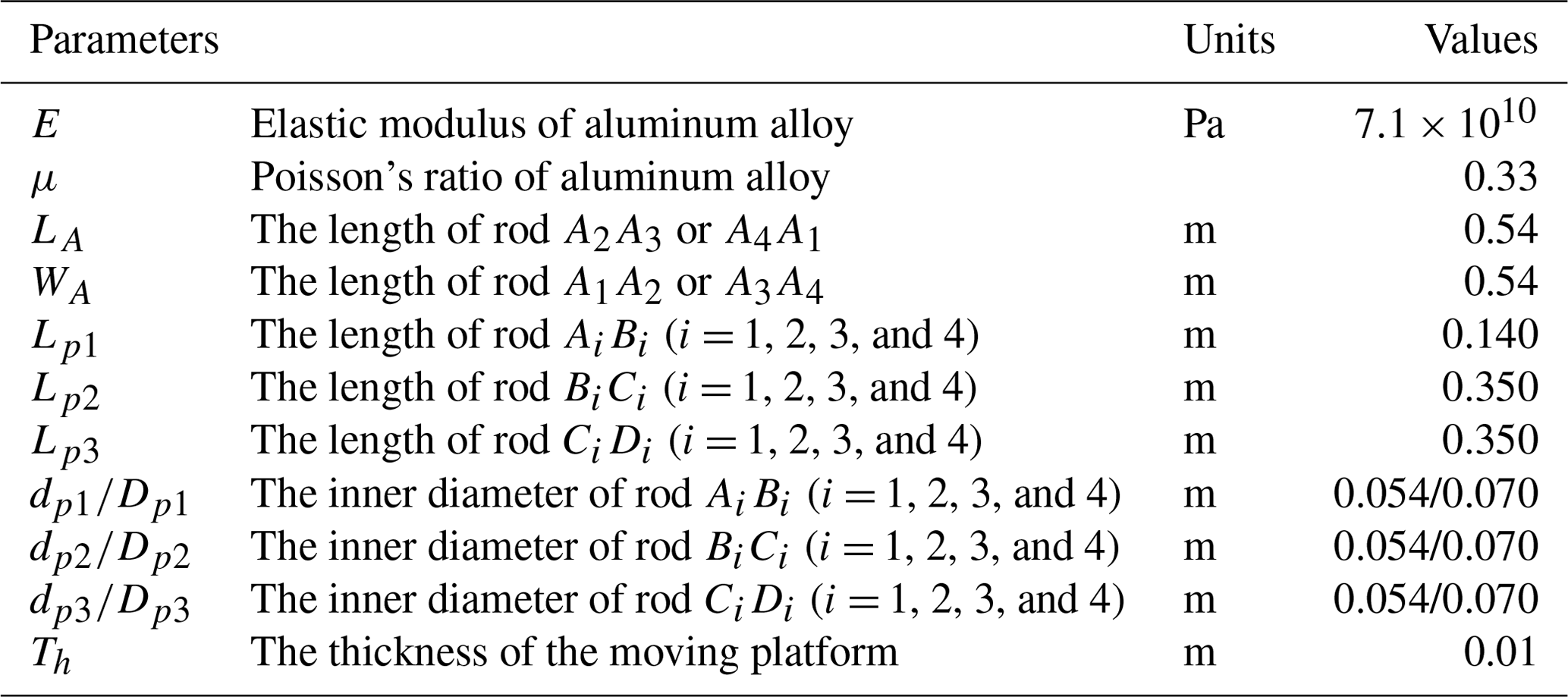
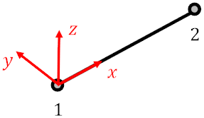
As shown in Fig. 1a, the quadruped wall-climbing robot (4SRRR parallel robot) is developed to meet the needs of unstructured on-site work requirements for large and complex structural components. The schematic diagram is shown in Fig. 1b; the robot consists of a moving platform, a fixed platform (when the quadruped wall-climbing robot reaches the working position, the fixed feet and the working wall form the fixed platform), and four identical SRRR limbs. The limbs are symmetrically distributed, and each limb comprises three active rotational joints (R) and one passive spherical joint (S). The parallel robot has a total of 12 active rotational joints as the input to the mechanism. The physical and structural parameters of the robot are shown in Table 1.

Figure 1 4SRRR parallel robot: (a) 3D design diagram, (b) mechanism schematic diagram.

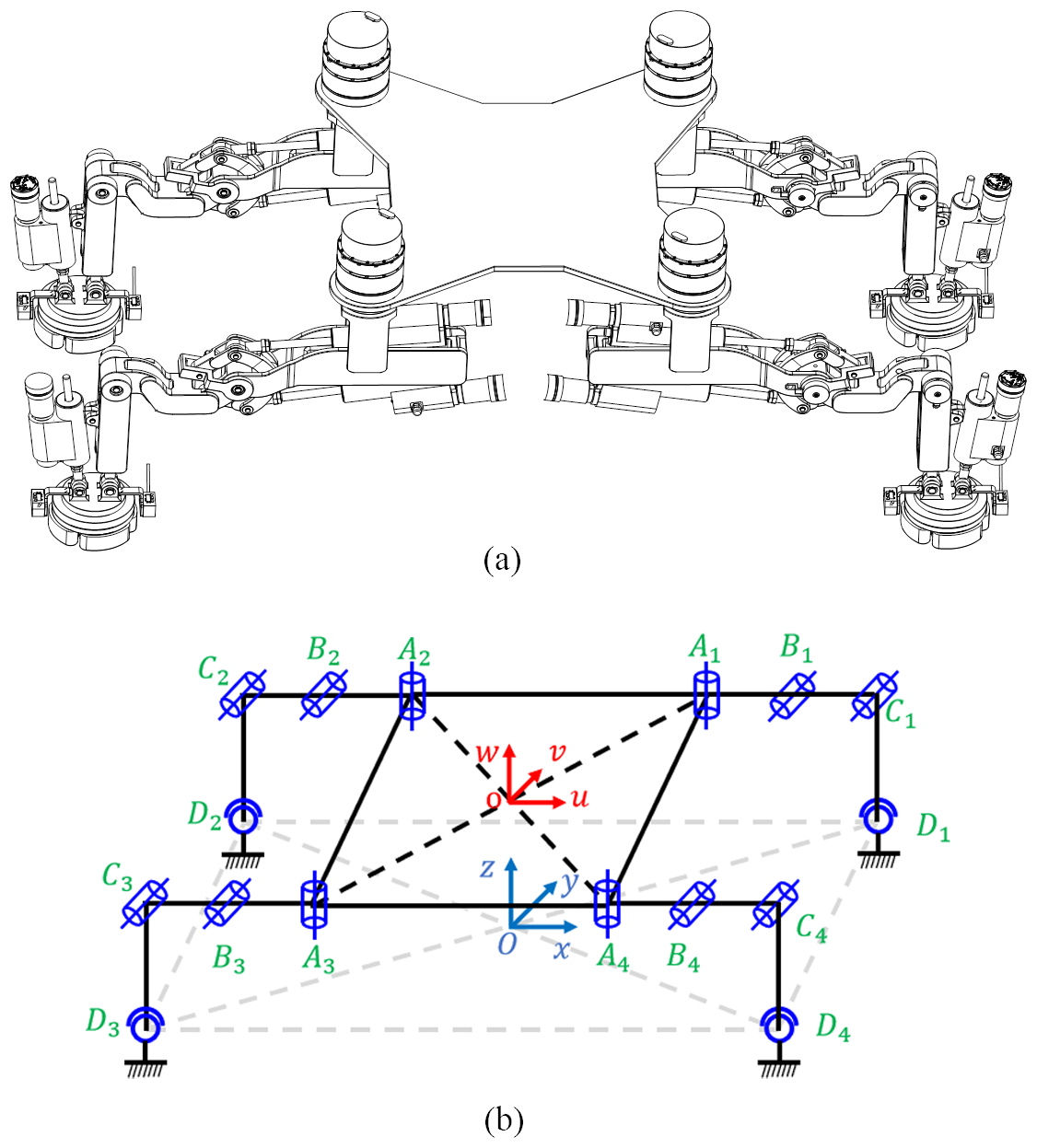
Table 1 Physical and structural parameters of the 4SRRR parallel robot.

The moving coordinate system {o−uvw} has its origin at the geometric center of the moving platform of the robot, the w axis is perpendicular to the plane of the moving platform, the u axis is parallel to the line connecting points A₃ and A₄, and the v axis is determined by the right-hand rule. The fixed coordinate system {O−xyz} has its origin at the geometric center of the fixed platform of the robot, the z axis points vertically upward, the x axis is parallel to the line connecting points D₃ and D₄, and the y axis is determined by the right-hand rule.

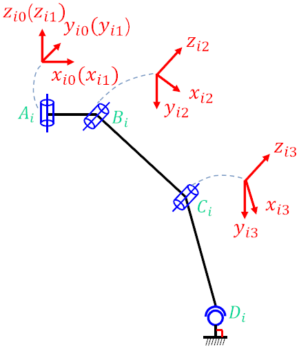
As shown in Fig. 2, the limbs of the robot are connected to the moving platform at points A_i via R joints (with axes perpendicular to the surface of the moving platform) and to the fixed platform at points D_i via S joints. The local coordinate systems {A_i−x_i1y_i1z_i1}, {B_i−x_i2y_i2z_i2}, and {C_i−x_i3y_i3z_i3} have their z_i1, z_i2, and z_i3 axes aligned along the axes of A_i, B_i, and C_i, respectively. The x_i1, x_i2, and x_i3 axes point in the directions of A_iB_i, B_iC_i, and C_iD_i, respectively.

Figure 2 Limb coordinate system of the 4SRRR parallel robot.

The foot must be perpendicular to the work surface due to the magnetic suction when the 4SRRR parallel robot is attracted to the work surface. Figure 3 illustrates the inverse kinematics calculation diagram of the limb of the 4SRRR parallel robot.

Figure 3 Inverse kinematics of the 4SRRR parallel robot.

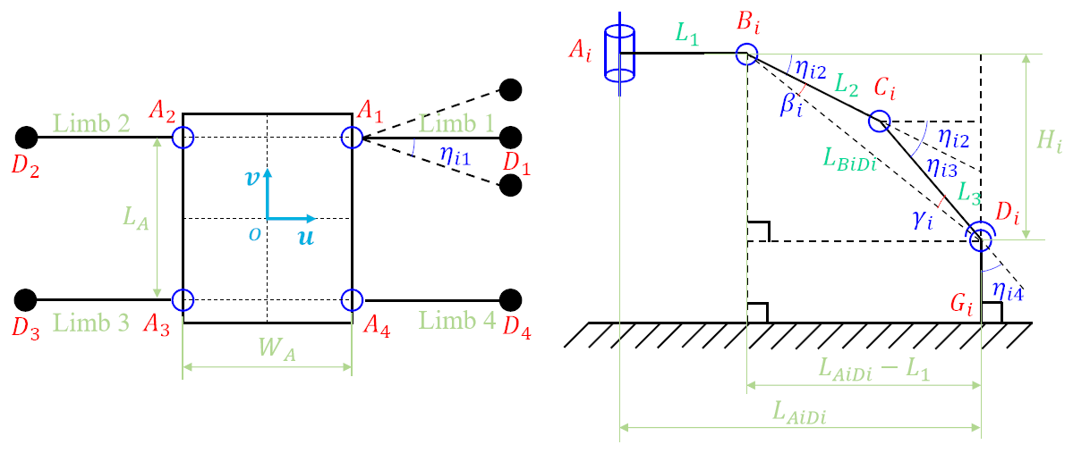
The coordinate of A_i in the moving coordinate system is (${}^o{u}_{A_i}$, ${}^o{v}_{A_i}$, ${}^o{w}_{A_i}$), and the coordinates of D_i is (${}^o{u}_{D_i}$, ${}^o{v}_{D_i}$, ${}^o{w}_{D_i}$). The following equation, according to the geometric relationships, is

$$\begin{array}{}\text{(1)}& \left\{\begin{array}{l}{\mathit{\eta }}_{i\mathrm{1}}=a\tan \mathrm{2}\left({}^o{v}_{D_i}{-}^o{v}_{A_i}{,}^o{u}_{D_i}{-}^o{u}_{A_i}\right),\\ L_{A_i{D}_i}=\text{abs}\left[\left({}^o{u}_{D_i}{-}^o{u}_{A_i}\right)/\cos \left({\mathit{\eta }}_{i\mathrm{1}}\right)\right],\\ H_i=\text{abs}\left({}^o{w}_{A_i}{-}^o{w}_{D_i}\right),\\ L_{B_i{D}_i}=\sqrt{{\left(L_{A_i{D}_i}-L_{\mathrm{1}}\right)}^{\mathrm{2}}+H_i^{\mathrm{2}}}.\end{array}\right.\end{array}$$

According to the cosine theorem,

$$\begin{array}{}\text{(2)}& \left\{\begin{array}{l}{\mathit{\eta }}_{\mathrm{3}i}=\mathit{\pi }-a\cos \left(\frac{L_{\mathrm{2}}^{\mathrm{2}}+L_{\mathrm{3}}^{\mathrm{2}}-L_{B_i{D}_i}^{\mathrm{2}}}{\mathrm{2}{L}_{\mathrm{2}}{L}_{\mathrm{3}}}\right),\\ {\mathit{\beta }}_i=a\cos \left(\frac{L_{\mathrm{2}}^{\mathrm{2}}+L_{B_i{D}_i}^{\mathrm{2}}-L_{\mathrm{3}}^{\mathrm{2}}}{\mathrm{2}{L}_{\mathrm{2}}{L}_{B_i{D}_i}}\right).\end{array}\right.\end{array}$$

Then,

$$\begin{array}{}\text{(3)}& {\mathit{\eta }}_{i\mathrm{2}}+{\mathit{\beta }}_i=a\tan \mathrm{2}\left(H_i,L_i-L_{\mathrm{1}}\right).\end{array}$$

We can then obtain

$$\begin{array}{}\text{(4)}& \left\{\begin{array}{l}{\mathit{\eta }}_{i\mathrm{2}}=a\tan \mathrm{2}\left(H_i,L_i-L_{\mathrm{1}}\right)-{\mathit{\beta }}_i,\\ {\mathit{\eta }}_{i\mathrm{4}}=\frac{\mathit{\pi }}{\mathrm{2}}-{\mathit{\eta }}_{i\mathrm{2}}-{\mathit{\eta }}_{i\mathrm{3}}.\end{array}\right.\end{array}$$

3 Elastodynamic model

The following assumptions are made for the parallel robot:

• 1.

  The fixed base, moving platform, motors, and all joints are rigid.

• 2.

  All joints are considered to be frictionless.

• 3.

  The rods are considered to be flexible, and the spatial composite deformation of the rods (including the tension (or compression), shear, torsional, and bending deformation components) is considered.

• 4.

  The deformation of all components is linear and within the elastic range.

3.1 Stiffness and mass matrices of one rod in the global coordinate

As shown in Fig. 4, the beam element has two nodal points at its ends, each possessing 6 degrees of freedom, resulting in a total of 12 degrees of freedom. The column vector of the nodal points, which represents the generalized coordinates of the beam element, can be expressed as ${\mathit{X}}_e={\left[{\mathit{d}}_{e\mathrm{1}},{\mathit{r}}_{e\mathrm{1}},{\mathit{d}}_{e\mathrm{2}},{\mathit{r}}_{e\mathrm{2}}\right]}^{\mathrm{T}}$, where d_e1 (r_e1) and d_e2 (r_e2) denote the translational (rotational) displacements of nodes 1 and 2, respectively, in the element's coordinate system.

Figure 4 Timoshenko beam element.

According to finite element theory, the stiffness matrix and the mass matrix of the beam element can be expressed as follows:

$$\begin{array}{}\text{(5)}& \left\{\begin{array}{l}{\mathbf{K}}_e=\int \underset{V_e}{\int }\int {\mathbf{B}}^{\mathrm{T}}\mathbf{DB}\text{d}V,\\ {\mathbf{M}}_e=\int \underset{V_e}{\int }\int \mathit{\rho }{\mathbf{N}}^{\mathrm{T}}\mathbf{N}\text{d}V,\end{array}\right.\end{array}$$

where K_e represents the element stiffness matrix; M_e represents the element mass matrix; V_e is the volume of the element; B is the strain-displacement transformation matrix and is given by ε_e=Bu_e, where ε_e=(ε_xε_yε_zγ_xyγ_yzγ_zx)^T is the strain column vector of the element; D denotes the elasticity matrix and is given by σ_e=Dε_e, where σ_e=(σ_xσ_yσ_zτ_xyτ_yzτ_zx)^T is the stress column vector of the element; ρ is the material density; and N is the shape function matrix and is given by X_ein=NX_e, where X_ein is the displacement column vector at any point within the element.

Constructing an element matrix that accurately reflects the true elastic deformation of the components is a key factor in establishing an accurate dynamic model of a parallel robot. To more precisely calculate the actual elastic deformation of the linkages, the beam element model employs a Timoshenko beam that accounts for shear deformation. The expressions for the element stiffness matrix and element mass matrix in the local coordinate system of the element can be derived as follows:

$$\begin{array}{}\text{(6)}& {\mathbf{K}}_e=\left(\begin{array}{cc}{\mathbf{K}}_{e\mathrm{11}}& {\mathbf{K}}_{e\mathrm{12}}\\ {\mathbf{K}}_{e\mathrm{12}}^{\mathrm{T}}& {\mathbf{K}}_{e\mathrm{22}}\end{array}\right),\end{array}$$

$$\begin{array}{}\text{(7)}& {\mathbf{M}}_e={\displaystyle \frac{\mathit{\rho }A{L}_e}{\mathrm{420}}}\left(\begin{array}{cc}{\mathbf{M}}_{e\mathrm{11}}& {\mathbf{M}}_{e\mathrm{12}}\\ {\mathbf{M}}_{e\mathrm{12}}^{\mathrm{T}}& {\mathbf{M}}_{e\mathrm{22}}\end{array}\right),\end{array}$$

where

$$\begin{array}{}\text{(8)}& {\mathbf{K}}_{e\mathrm{11}}=\left(\begin{array}{cccccc}{\displaystyle \frac{EA}{L_e}}& \mathrm{0}& \mathrm{0}& \mathrm{0}& \mathrm{0}& \mathrm{0}\\ \mathrm{0}& \frac{\mathrm{12}EG{I}_z{A}_y}{L_e{g}_{\mathrm{1}}}& \mathrm{0}& \mathrm{0}& \mathrm{0}& \frac{\mathrm{6}EG{I}_z{A}_y}{g_{\mathrm{1}}}\\ \mathrm{0}& \mathrm{0}& \frac{\mathrm{12}EG{I}_y{A}_z}{L_e{g}_{\mathrm{2}}}& \mathrm{0}& -\frac{\mathrm{6}EG{I}_y{A}_z}{g_{\mathrm{2}}}& \mathrm{0}\\ \mathrm{0}& \mathrm{0}& \mathrm{0}& \frac{G{I}_p}{L_e}& \mathrm{0}& \mathrm{0}\\ \mathrm{0}& \mathrm{0}& -\frac{\mathrm{6}EG{I}_y{A}_z}{g_{\mathrm{2}}}& \mathrm{0}& \frac{\mathrm{4}E{I}_y{b}_{\mathrm{1}}}{L_e{g}_{\mathrm{2}}}& \mathrm{0}\\ \mathrm{0}& \frac{\mathrm{6}EG{I}_z{A}_y}{g_{\mathrm{1}}}& \mathrm{0}& \mathrm{0}& \mathrm{0}& \frac{\mathrm{4}E{I}_z{b}_{\mathrm{2}}}{L_e{g}_{\mathrm{1}}}\end{array}\right),\end{array}$$

$$\begin{array}{}\text{(9)}& {\mathbf{K}}_{e\mathrm{12}}=\left(\begin{array}{cccccc}-{\displaystyle \frac{EA}{L_e}}& \mathrm{0}& \mathrm{0}& \mathrm{0}& \mathrm{0}& \mathrm{0}\\ \mathrm{0}& -\frac{\mathrm{12}EG{I}_z{A}_y}{L_e{g}_{\mathrm{1}}}& \mathrm{0}& \mathrm{0}& \mathrm{0}& \frac{\mathrm{6}EG{I}_z{A}_y}{g_{\mathrm{1}}}\\ \mathrm{0}& \mathrm{0}& -\frac{\mathrm{12}EG{I}_y{A}_z}{L_e{g}_{\mathrm{2}}}& \mathrm{0}& -\frac{\mathrm{6}EG{I}_y{A}_z}{g_{\mathrm{2}}}& \mathrm{0}\\ \mathrm{0}& \mathrm{0}& \mathrm{0}& -\frac{G{I}_p}{L_e}& \mathrm{0}& \mathrm{0}\\ \mathrm{0}& \mathrm{0}& \frac{\mathrm{6}EG{I}_y{A}_z}{g_{\mathrm{2}}}& \mathrm{0}& \frac{\mathrm{6}EG{I}_y{A}_z{L}_e}{g_{\mathrm{2}}}-\frac{\mathrm{4}E{I}_y{b}_{\mathrm{1}}}{L_e{g}_{\mathrm{2}}}& \mathrm{0}\\ \mathrm{0}& -\frac{\mathrm{6}EG{I}_z{A}_y}{g_{\mathrm{1}}}& \mathrm{0}& \mathrm{0}& \mathrm{0}& \frac{\mathrm{6}EG{I}_z{A}_y{L}_e}{g_{\mathrm{1}}}-\frac{\mathrm{4}E{I}_z{b}_{\mathrm{2}}}{L_e{g}_{\mathrm{1}}}\end{array}\right),\end{array}$$

$$\begin{array}{}\text{(10)}& {\mathbf{K}}_{e\mathrm{22}}=\left(\begin{array}{cccccc}\frac{EA}{L_e}& \mathrm{0}& \mathrm{0}& \mathrm{0}& \mathrm{0}& \mathrm{0}\\ \mathrm{0}& \frac{\mathrm{12}EG{I}_z{A}_y}{L_e{g}_{\mathrm{1}}}& \mathrm{0}& \mathrm{0}& \mathrm{0}& -\frac{\mathrm{6}EG{I}_z{A}_y}{g_{\mathrm{1}}}\\ \mathrm{0}& \mathrm{0}& \frac{\mathrm{12}EG{I}_y{A}_z}{L_e{g}_{\mathrm{2}}}& \mathrm{0}& \frac{\mathrm{6}EG{I}_y{A}_z}{g_{\mathrm{2}}}& \mathrm{0}\\ \mathrm{0}& \mathrm{0}& \mathrm{0}& \frac{G{I}_p}{L_e}& \mathrm{0}& \mathrm{0}\\ \mathrm{0}& \mathrm{0}& \frac{\mathrm{6}EG{I}_y{A}_z}{g_{\mathrm{2}}}& \mathrm{0}& \frac{\mathrm{4}E{I}_y{b}_{\mathrm{1}}}{L_e{g}_{\mathrm{2}}}& \mathrm{0}\\ \mathrm{0}& -\frac{\mathrm{6}EG{I}_z{A}_y}{g_{\mathrm{1}}}& \mathrm{0}& \mathrm{0}& \mathrm{0}& \frac{\mathrm{4}E{I}_z{b}_{\mathrm{2}}}{L_e{g}_{\mathrm{1}}}\end{array}\right),\end{array}$$

$$\begin{array}{}\text{(11)}& {\mathbf{M}}_{e\mathrm{11}}=\left(\begin{array}{cccccc}\mathrm{140}& \mathrm{0}& \mathrm{0}& \mathrm{0}& \mathrm{0}& \mathrm{0}\\ \mathrm{0}& \mathrm{156}& \mathrm{0}& \mathrm{0}& \mathrm{0}& \mathrm{22}{L}_e\\ \mathrm{0}& \mathrm{0}& \mathrm{156}& \mathrm{0}& -\mathrm{22}{L}_e& \mathrm{0}\\ \mathrm{0}& \mathrm{0}& \mathrm{0}& \mathrm{140}{I}_p/A& \mathrm{0}& \mathrm{0}\\ \mathrm{0}& \mathrm{0}& -\mathrm{22}{L}_e& \mathrm{0}& \mathrm{4}{L}_e^{\mathrm{2}}& \mathrm{0}\\ \mathrm{0}& \mathrm{22}{L}_e& \mathrm{0}& \mathrm{0}& \mathrm{0}& \mathrm{4}{L}_e^{\mathrm{2}}\end{array}\right),\end{array}$$

$$\begin{array}{}\text{(12)}& {\mathbf{M}}_{e\mathrm{12}}=\left(\begin{array}{cccccc}\mathrm{70}& \mathrm{0}& \mathrm{0}& \mathrm{0}& \mathrm{0}& \mathrm{0}\\ \mathrm{0}& \mathrm{54}& \mathrm{0}& \mathrm{0}& \mathrm{0}& -\mathrm{13}{L}_e\\ \mathrm{0}& \mathrm{0}& \mathrm{54}& \mathrm{0}& \mathrm{13}{L}_e& \mathrm{0}\\ \mathrm{0}& \mathrm{0}& \mathrm{0}& \mathrm{70}{I}_p/A& \mathrm{0}& \mathrm{0}\\ \mathrm{0}& \mathrm{0}& -\mathrm{13}{L}_e& \mathrm{0}& -\mathrm{3}{L}_e^{\mathrm{2}}& \mathrm{0}\\ \mathrm{0}& \mathrm{13}{L}_e& \mathrm{0}& \mathrm{0}& \mathrm{0}& -\mathrm{3}{L}_e^{\mathrm{2}}\end{array}\right),\end{array}$$

$$\begin{array}{}\text{(13)}& {\mathbf{M}}_{e\mathrm{22}}=\left(\begin{array}{cccccc}\mathrm{140}& \mathrm{0}& \mathrm{0}& \mathrm{0}& \mathrm{0}& \mathrm{0}\\ \mathrm{0}& \mathrm{156}& \mathrm{0}& \mathrm{0}& \mathrm{0}& -\mathrm{22}{L}_e\\ \mathrm{0}& \mathrm{0}& \mathrm{156}& \mathrm{0}& \mathrm{22}{L}_e& \mathrm{0}\\ \mathrm{0}& \mathrm{0}& \mathrm{0}& \mathrm{140}{I}_p/A& \mathrm{0}& \mathrm{0}\\ \mathrm{0}& \mathrm{0}& \mathrm{22}{L}_e& \mathrm{0}& \mathrm{4}{L}_e^{\mathrm{2}}& \mathrm{0}\\ \mathrm{0}& -\mathrm{22}{L}_e& \mathrm{0}& \mathrm{0}& \mathrm{0}& \mathrm{4}{L}_e^{\mathrm{2}}\end{array}\right),\end{array}$$

where G is the shear modulus; I_x and I_y are the moments of inertia of the cross-section about the x and y axes, respectively; I_p and A represent the polar moment of inertia and the area of the cross-section, respectively; A_y and A_z are the effective shear areas of the cross-section along the y and z axis, respectively; L_e represents the length of the beam element; and $g_{\mathrm{1}}=G{A}_y{L}^{\mathrm{2}}+\mathrm{12}E{I}_z$, $g_{\mathrm{2}}=G{A}_z{L}^{\mathrm{2}}+\mathrm{12}E{I}_y$, $b_{\mathrm{1}}=G{A}_z{L}^{\mathrm{2}}+\mathrm{3}E{I}_y$, and $b_{\mathrm{2}}=G{A}_y{L}^{\mathrm{2}}+\mathrm{3}E{I}_z$.

The kinetic energy and elastic potential energy of the beam element can be expressed as follows:

$$\begin{array}{}\text{(14)}& \left\{\begin{array}{l}{E}_{\mathrm{ke}}=\frac{\mathrm{1}}{\mathrm{2}}{\dot{\mathit{X}}}_e^{\mathrm{T}}{\mathbf{M}}_e{\dot{\mathit{X}}}_e,\\ E_{\mathrm{pe}}=\frac{\mathrm{1}}{\mathrm{2}}{\mathit{X}}_e^{\mathrm{T}}{\mathbf{K}}_e{\mathit{X}}_e,\end{array}\right.\end{array}$$

where E_ke and E_pe represent the kinetic energy and elastic potential energy of the beam element, respectively.

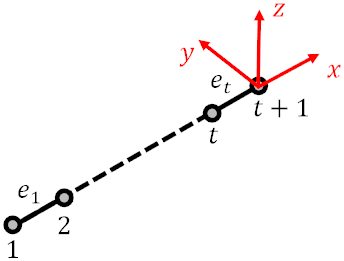
As shown in Fig. 5, considering the jth rod in limb i divided into t elements, where $e_k(k=\mathrm{1},\mathrm{\dots },t)$ represents the kth element, the generalized displacement coordinates of the jth rod of limb i can be expressed as follows:

$$\begin{array}{}\text{(15)}& {}^L{\mathit{X}}_{i,j}={\left({{}^L}_{i,j,\mathrm{1}}{{,}^L}_{i,j,\mathrm{2}},\mathrm{\dots }{{,}^L}_{i,j,t+\mathrm{1}}\right)}_{\mathrm{6}(t+\mathrm{1})\times \mathrm{1}}^{\mathrm{T}},\end{array}$$

where ${}^L{\mathit{X}}_{r,i,j}$ represents the generalized displacement coordinates of the jth rod in limb i; the superscript “L” indicates that the vector is expressed in the local coordinate system; and ${}^L{\mathit{X}}_k(k=\mathrm{1},\mathrm{\dots },t+\mathrm{1})$ denotes the displacement coordinates of the kth node of the jth rod in limb i.

Figure 5 Finite element model of a rod.

The mapping relationship between the displacement coordinates ${}^L{\mathit{X}}_{e,i,j,k}$ of the kth node of the jth rod in limb i and the generalized displacement coordinates ^LX_i,j of the rod can be written as follows:

$$\begin{array}{}\text{(16)}& {}^L{\mathit{X}}_{e,i,j,k}={\mathbf{T}}_{e,i,j,k}^L{\mathit{X}}_{i,j}\end{array}$$

where ${}^L{\mathit{X}}_{e,i,j,k}=\left({}^L{\mathit{X}}_{i,j,k}^L{\mathit{X}}_{i,j,k+\mathrm{1}}\right)$ represents the displacement coordinates of the kth element of the jth rod in limb i in the local coordinate system, and ${\mathbf{T}}_{e,i,j,k}$ denotes the mapping matrix from the generalized displacement coordinates of the jth rod in limb i to the displacement coordinates of the kth element of the jth rod in limb i. Furthermore, we have

$$\begin{array}{}\text{(17)}& \left\{\begin{array}{l}{\mathbf{T}}_{e,i,j,\mathrm{1}}={\left(\begin{array}{ccc}{\mathbf{E}}_{\mathrm{6}}& {\mathrm{0}}_{\mathrm{6}}& \mathrm{\cdots }\\ {\mathrm{0}}_{\mathrm{6}}& {\mathbf{E}}_{\mathrm{6}}& \mathrm{\cdots }\end{array}\right)}_{\mathrm{12}\times (\mathrm{6}t+\mathrm{6})},\\ {\mathbf{T}}_{e,i,j,\mathrm{2}}={\left(\begin{array}{cccc}{\mathrm{0}}_{\mathrm{6}}& {\mathbf{E}}_{\mathrm{6}}& {\mathrm{0}}_{\mathrm{6}}& \mathrm{\cdots }\\ {\mathrm{0}}_{\mathrm{6}}& {\mathrm{0}}_{\mathrm{6}}& {\mathbf{E}}_{\mathrm{6}}& \mathrm{\cdots }\end{array}\right)}_{\mathrm{12}\times (\mathrm{6}t+\mathrm{6})},\\ \mathrm{⋮}\mathrm{⋮}\\ {\mathbf{T}}_{e,i,j,t}={\left(\begin{array}{cccc}{\mathrm{0}}_{\mathrm{6}}& \mathrm{\cdots }& {\mathbf{E}}_{\mathrm{6}}& {\mathrm{0}}_{\mathrm{6}}\\ {\mathrm{0}}_{\mathrm{6}}& \mathrm{\cdots }& {\mathrm{0}}_{\mathrm{6}}& {\mathbf{E}}_{\mathrm{6}}\end{array}\right)}_{\mathrm{12}\times (\mathrm{6}t+\mathrm{6})},\end{array}\right.\end{array}$$

where E₆ is a 6 × 6 identity matrix, and 0₆ is a 6 × 6 zero matrix.

The kinetic energy and elastic potential energy of the e_k element, based on the generalized displacement coordinates of rod j of limb i, can be expressed as follows:

$$\begin{array}{}\text{(18)}& \left\{\begin{array}{l}\begin{array}{rl}& E_{e,i,j,k}^{\mathrm{ke}}\\ & ={\displaystyle \frac{\mathrm{1}}{\mathrm{2}}}{}^L{\dot{\mathit{X}}}_{e,i,j,k}^{\mathrm{T}}{}^L{\mathbf{M}}_{e,i,j,k}^L{\dot{\mathit{X}}}_{e,i,j,k}\\ & ={\displaystyle \frac{\mathrm{1}}{\mathrm{2}}}{}^L{\dot{\mathit{X}}}_{i,j}^{\mathrm{T}}{\mathbf{T}}_{e,i,j,k}^{\mathrm{T}}{}^L{\mathbf{M}}_{e,i,j,k}{\mathbf{T}}_{e,i,j,k}^L{\dot{\mathit{X}}}_{i,j}\\ & ={\displaystyle \frac{\mathrm{1}}{\mathrm{2}}}{}^L{\dot{\mathit{X}}}_{i,j}^{\mathrm{T}}{}^L{\mathbf{M}}_{e,i,j,k}^{\mathrm{r}}{}^L{\dot{\mathit{X}}}_{i,j},\end{array}\\ \\ \begin{array}{rl}& E_{e,i,j,k}^{\mathrm{pe}}\\ & ={\displaystyle \frac{\mathrm{1}}{\mathrm{2}}}{}^L{\mathit{X}}_{e,i,j,k}^{\mathrm{T}}{}^L{\mathbf{K}}_{e,i,j,k}^L{\mathit{X}}_{e,i,j,k}\\ & ={\displaystyle \frac{\mathrm{1}}{\mathrm{2}}}{}^L{\mathit{X}}_{i,j}^{\mathrm{T}}{\mathbf{T}}_{e,i,j,k}^{\mathrm{T}}{}^L{\mathbf{K}}_{e,i,j,k}{\mathbf{T}}_{e,i,j,k}^L{\mathit{X}}_{i,j}\\ & ={\displaystyle \frac{\mathrm{1}}{\mathrm{2}}}{}^L{\mathit{X}}_{i,j}^{\mathrm{T}}{}^L{\mathbf{K}}_{e,i,j,k}^{\mathrm{r}}{}^L{\mathit{X}}_{i,j},\end{array}\end{array}\right.(k=\mathrm{1},\mathrm{\cdots },t)\end{array}$$

where ${}^L{\mathbf{M}}_{e,i,j,k}^{\mathrm{r}}={\mathbf{T}}_{e,i,j,k}^{\mathrm{T}}{}^L{\mathbf{M}}_{e,i,j,k}{\mathbf{T}}_{e,i,j,k}$ and ${}^L{\mathbf{K}}_{e,i,j,k}^{\mathrm{r}}={\mathbf{T}}_{e,i,j,k}^{\mathrm{T}}{}^L{\mathbf{K}}_{e,i,j,k}{\mathbf{T}}_{e,i,j,k}$ represent the mass contribution matrix and stiffness contribution matrix of the kth element of the jth rod in limb i, respectively.

Summing over Eq. (18) yields the kinetic energy and elastic potential energy of a single rod:

$$\begin{array}{}\text{(19)}& \left\{\begin{array}{l}\begin{array}{rl}{E}_{\mathrm{ke},i,j}& =\sum _{k=\mathrm{1}}^t{E}_{e,i,j,k}^{\mathrm{ke}}={\displaystyle \frac{\mathrm{1}}{\mathrm{2}}}{}^L{\dot{\mathit{X}}}_{i,j}^{\mathrm{T}}\left(\sum _{k=\mathrm{1}}^t{}^L{\mathbf{M}}_{e,i,j,k}^{\mathrm{r}}\right){}^L{\dot{\mathit{X}}}_{i,j}\\ & ={\displaystyle \frac{\mathrm{1}}{\mathrm{2}}}{}^L{\dot{\mathit{X}}}_{i,j}^{\mathrm{T}}{}^L{\mathbf{M}}_{i,j}^L{\dot{\mathit{X}}}_{i,j},\\ E_{\mathrm{pe},i,j}& =\sum _{k=\mathrm{1}}^t{E}_{e,i,j,k}^{\mathrm{pe}}={\displaystyle \frac{\mathrm{1}}{\mathrm{2}}}{}^L{\mathit{X}}_{i,j}^{\mathrm{T}}\left(\sum _{k=\mathrm{1}}^t{}^L{\mathbf{K}}_{e,i,j,k}^{\mathrm{r}}\right){}^L{\mathit{X}}_{i,j}\\ & ={\displaystyle \frac{\mathrm{1}}{\mathrm{2}}}{}^L{\mathit{X}}_{i,j}^{\mathrm{T}}{}^L{\mathbf{K}}_{i,j}^L{\mathit{X}}_{i,j},\end{array}\end{array}\right.\end{array}$$

where ${}^L{\mathbf{M}}_{i,j}=\sum _{k=\mathrm{1}}^t{}^L{\mathbf{M}}_{e,i,j,k}^{\mathrm{r}}$ and ${}^L{\mathbf{K}}_{i,j}=\sum _{k=\mathrm{1}}^t{}^L{\mathbf{K}}_{e,i,j,k}^{\mathrm{r}}$ represent the mass matrix and stiffness matrix of the rod in the local coordinate system, respectively.

The transformation matrix between the generalized displacement coordinates of the jth rod in limb i in the local coordinate system and the global coordinate system is defined as follows:

$$\begin{array}{}\text{(20)}& {\dot{\mathit{X}}}_{i,j}={\mathbf{D}}_{i,j}^L{\dot{\mathit{X}}}_{i,j},\end{array}$$

where ${\mathbf{D}}_{i,j}=\text{diag}{\left[{\mathbf{R}}_{i,j},\mathrm{\dots },{\mathbf{R}}_{i,j}\right]}^{\mathrm{T}}$, and R_i,j represents the transformation matrix between the local coordinate system and the global coordinate system of the jth rod in limb i.

By substituting Eq. (20) into Eq. (19), the expressions for the kinetic and potential energy of rod j of limb i based on X_i,j can be derived as follows:

$$\begin{array}{}\text{(21)}& \left\{\begin{array}{l}{E}_{\mathrm{ke},i,j}=\frac{\mathrm{1}}{\mathrm{2}}{\dot{\mathit{X}}}_{i,j}^{\mathrm{T}}{\mathbf{D}}_{i,j}^{\mathrm{T}}{}^L{\mathbf{M}}_{i,j}{\mathbf{D}}_{i,j}{\dot{\mathit{X}}}_{i,j}=\frac{\mathrm{1}}{\mathrm{2}}{\dot{\mathit{X}}}_{i,j}^{\mathrm{T}}{\mathbf{M}}_{i,j}{\dot{\mathit{X}}}_{i,j},\\ E_{\mathrm{pe},i,j}=\frac{\mathrm{1}}{\mathrm{2}}{\mathit{X}}_{i,j}^{\mathrm{T}}{\mathbf{D}}_{i,j}^{\mathrm{T}}{}^L{\mathbf{K}}_{i,j}{\mathbf{D}}_{i,j}{\mathit{X}}_{i,j}=\frac{\mathrm{1}}{\mathrm{2}}{\mathit{X}}_{i,j}^{\mathrm{T}}{\mathbf{K}}_{i,j}{\mathit{X}}_{i,j},\end{array}\right.\end{array}$$

where ${\mathbf{M}}_{i,j}={\mathbf{D}}_{i,j}^L{\mathbf{M}}_{i,j}{\mathbf{D}}_{i,j}^{\mathrm{T}}$ and ${\mathbf{K}}_{i,j}={\mathbf{D}}_{i,j}^L{\mathbf{K}}_{i,j}{\mathbf{D}}_{i,j}^{\mathrm{T}}$ represent the mass matrix and stiffness matrix of the jth rod in limb i in the global coordinate system, respectively.

3.2 Mass matrix of the moving platform in the global coordinate system

Assuming the moving platform is rigid (Yu and Chen, 2019; Lochan et al., 2018), the kinetic energy of the moving platform can be obtained using the aforementioned method:

$$\begin{array}{}\text{(22)}& E_{\mathrm{ko}}={\displaystyle \frac{\mathrm{1}}{\mathrm{2}}}{}^o{\dot{\mathit{X}}}_o^{\mathrm{T}}{}^o{\mathbf{M}}_o^o{\dot{\mathit{X}}}_o={\displaystyle \frac{\mathrm{1}}{\mathrm{2}}}{\dot{\mathit{X}}}_o^{\mathrm{T}}{\mathbf{D}}_o^o{\mathbf{M}}_o{\mathbf{D}}_o^{\mathrm{T}}{\dot{\mathit{X}}}_o={\displaystyle \frac{\mathrm{1}}{\mathrm{2}}}{\dot{\mathit{X}}}_o^{\mathrm{T}}{\mathbf{M}}_o{\dot{\mathit{X}}}_o,\end{array}$$

${\mathit{X}}_o={\left({\mathit{d}}_o,{\mathit{r}}_o\right)}^{\mathrm{T}}$ and ^oX_o represent the displacement arrays of the exit node o of the moving platform in the global coordinate system and the local coordinate system {o}, respectively; M_o and ^oM_o represent the mass matrix of the moving platform in the global coordinate system and the local coordinate system, respectively; and ${\mathbf{D}}_o=\text{diag}\left[\mathbf{R},\mathbf{R}\right]$ is the transformation matrix for the displacement vector of the exit node of the moving platform between the local coordinate system and the global coordinate system.

By using Eq. (22), we can obtain

$$\begin{array}{}\text{(23)}& {\mathbf{M}}_o={\mathbf{D}}_o^o{\mathbf{M}}_o{\mathbf{D}}_o^{\mathrm{T}}.\end{array}$$

3.3 Mass and stiffness matrices of the parallel robot in the global coordinate system

The global independent extended generalized displacement coordinates of the 4SRRR parallel robot can be expressed as

$$\begin{array}{}\text{(24)}& \begin{array}{rl}\mathit{X}& =[{\mathit{X}}_{C_{\mathrm{1}}{D}_{\mathrm{1}}}^{\mathrm{T}},{\mathit{X}}_{B_{\mathrm{1}}{C}_{\mathrm{1}}}^{\mathrm{T}},{\mathit{X}}_{A_{\mathrm{1}}{B}_{\mathrm{1}}}^{\mathrm{T}},{\mathit{X}}_{C_{\mathrm{2}}{D}_{\mathrm{2}}}^{\mathrm{T}},{\mathit{X}}_{B_{\mathrm{2}}{C}_{\mathrm{2}}}^{\mathrm{T}},{\mathit{X}}_{A_{\mathrm{2}}{B}_{\mathrm{2}}}^{\mathrm{T}},\\ & {\mathit{X}}_{C_{\mathrm{3}}{D}_{\mathrm{3}}}^{\mathrm{T}},{\mathit{X}}_{B_{\mathrm{3}}{C}_{\mathrm{3}}}^{\mathrm{T}},{\mathit{X}}_{A_{\mathrm{3}}{B}_{\mathrm{3}}}^{\mathrm{T}},{\mathit{X}}_{C_{\mathrm{4}}{D}_{\mathrm{4}}}^{\mathrm{T}},{\mathit{X}}_{B_{\mathrm{4}}{C}_{\mathrm{4}}}^{\mathrm{T}},{\mathit{X}}_{A_{\mathrm{4}}{B}_{\mathrm{4}}}^{\mathrm{T}},{\mathit{X}}_o{]}^{\mathrm{T}},\end{array}\end{array}$$

where ${\mathit{X}}_{A_i{B}_i}$, ${\mathit{X}}_{B_i{C}_i}$, and ${\mathit{X}}_{C_i{D}_i}$ represent the global independent generalized displacement coordinates of rods A_iB_i, B_iC_i, and C_iD_i in limb i, respectively.

The limbs of the 4SRRR parallel robot are connected to the moving platform, between limbs, and to the fixed platform through different joints. The exit nodes of the elements at the connections must satisfy certain constraint conditions. Therefore, the extended generalized displacement coordinates alone are insufficient to describe the physical properties of the mechanism; the constraint equations must be combined to extract the global independent generalized displacement coordinates of the mechanism. Correct extraction of the global independent generalized coordinates under different joint constraints is key to establishing an accurate dynamic model of the parallel robot.

Given the assumption that the moving platform is a rigid body, we have ${\mathit{r}}_{A_i}={\mathit{r}}_o$. Additionally, considering that all three active joints (R joints) of the 4SRRR parallel robot are locked, the boundary conditions at A_i for limb i can be expressed as

$$\begin{array}{}\text{(25)}& {\mathit{X}}_{A_i}=\left[\begin{array}{c}{\mathit{d}}_{A_i}\\ {\mathit{r}}_{A_i}\end{array}\right]=\left[\begin{array}{cc}{\mathbf{E}}_{\mathrm{3}}& \left[A_i\mathit{o}\times \right]\\ {\mathbf{\text{0}}}_{\mathrm{3}}& {\mathbf{E}}_{\mathrm{3}}\end{array}\right]{\mathit{X}}_o,\end{array}$$

where E₃ is a 3 × 3 identity matrix, and [A_io×] denotes the skew-symmetric matrix.

Similarly, rods A_iB_i and B_iC_i, as well as rods B_iC_i and C_iD_i, are connected at B_i and C_i through R joints. If all three active joints (R joints) of the 4SRRR parallel robot are locked, the boundary conditions at B_i and C_i for limb i can be expressed as

$$\begin{array}{}\text{(26)}& \left\{\begin{array}{l}{\mathit{X}}_{A_i{B}_i,B_i}={\mathit{X}}_{B_i{C}_i,B_i}={\mathit{X}}_{B_i},\\ {\mathit{X}}_{B_i{C}_i,C_i}={\mathit{X}}_{C_i{D}_i,C_i}={\mathit{X}}_{C_i}.\end{array}\right.\end{array}$$

Rod C_iD_i is connected to the fixed platform at D_i through an S joint. Based on the deformation characteristics of the S joint, the boundary conditions are given as follows:

$$\begin{array}{}\text{(27)}& {}^{D_i}{\mathit{d}}_{D_i}={\mathrm{0}}_{\mathrm{3}\times \mathrm{1}}.\end{array}$$

Since the S joint coordinate system {D_i−x_iy_iz_i} is parallel to the global coordinate system {O−xyz}, the boundary conditions at D_i for the limb are expressed the same way in both the global coordinate system and the local coordinate system. Thus, we have

$$\begin{array}{}\text{(28)}& {\mathit{d}}_{D_i}={\mathrm{0}}_{\mathrm{3}\times \mathrm{1}}.\end{array}$$

Based on the above analysis, the global independent generalized displacement coordinates of the 4SRRR parallel robot are defined as

$$\begin{array}{}\text{(29)}& \begin{array}{rl}\mathit{X}& =({\mathit{r}}_{D_{\mathrm{1}}}^{\mathrm{T}},{\mathit{X}}_{C_{\mathrm{1}}{D}_{\mathrm{1}},\mathrm{in}}^{\mathrm{T}},{\mathit{X}}_{C_{\mathrm{1}}}^{\mathrm{T}},{\mathit{X}}_{B_{\mathrm{1}}{C}_{\mathrm{1}},\mathrm{in}}^{\mathrm{T}},{\mathit{X}}_{B_{\mathrm{1}}}^{\mathrm{T}},{\mathit{X}}_{A_{\mathrm{1}}{B}_{\mathrm{1}},\mathrm{in}}^{\mathrm{T}},\\ & {\mathit{r}}_{D_{\mathrm{2}}}^{\mathrm{T}},{\mathit{X}}_{C_{\mathrm{2}}{D}_{\mathrm{2}},\mathrm{in}}^{\mathrm{T}},{\mathit{X}}_{C_{\mathrm{2}}}^{\mathrm{T}},{\mathit{X}}_{B_{\mathrm{2}}{C}_{\mathrm{2}},\mathrm{in}}^{\mathrm{T}},{\mathit{X}}_{B_{\mathrm{2}}}^{\mathrm{T}},{\mathit{X}}_{A_{\mathrm{2}}{B}_{\mathrm{2}},\mathrm{in}}^{\mathrm{T}},{\mathit{r}}_{D_{\mathrm{3}}}^{\mathrm{T}},\\ & {\mathit{X}}_{C_{\mathrm{3}}{D}_{\mathrm{3}},\mathrm{in}}^{\mathrm{T}},{\mathit{X}}_{C_{\mathrm{3}}}^{\mathrm{T}},{\mathit{X}}_{B_{\mathrm{3}}{C}_{\mathrm{3}},\mathrm{in}}^{\mathrm{T}},{\mathit{X}}_{B_{\mathrm{3}}}^{\mathrm{T}},{\mathit{X}}_{A_{\mathrm{3}}{B}_{\mathrm{3}},\mathrm{in}}^{\mathrm{T}},{\mathit{r}}_{D_{\mathrm{4}}}^{\mathrm{T}},\\ & {\mathit{X}}_{C_{\mathrm{4}}{D}_{\mathrm{4}},\mathrm{in}}^{\mathrm{T}},{\mathit{X}}_{C_{\mathrm{4}}}^{\mathrm{T}},{\mathit{X}}_{B_{\mathrm{4}}{C}_{\mathrm{4}},\mathrm{in}}^{\mathrm{T}},{\mathit{X}}_{B_{\mathrm{4}}}^{\mathrm{T}},{\mathit{X}}_{A_{\mathrm{4}}{B}_{\mathrm{4}},\mathrm{in}}^{\mathrm{T}},{\mathit{X}}_o^{\mathrm{T}}{)}^{\mathrm{T}}.\end{array}\end{array}$$

By combining Eqs. (24) and (29), the mapping relationship between the displacement coordinates of the rods and the moving platform with the global generalized displacement coordinates can be obtained:

$$\begin{array}{}\text{(30)}& \left\{\begin{array}{l}{\mathit{X}}_{i,\mathrm{1}}={\mathit{X}}_{C_i{D}_i}={\left({\mathit{X}}_{D_i}^{\mathrm{T}},{\mathit{X}}_{C_i{D}_i,\mathrm{in}}^{\mathrm{T}},{\mathit{X}}_{C_i}^{\mathrm{T}}\right)}^{\mathrm{T}}={\mathbf{\Gamma }}_{i,\mathrm{1}}\mathit{X}\\ (i=\mathrm{1},\mathrm{2},\mathrm{3},\mathrm{4}),\\ {\mathit{X}}_{i,\mathrm{2}}={\mathit{X}}_{B_i{C}_i}={\left({\mathit{X}}_{C_i}^{\mathrm{T}},{\mathit{X}}_{B_i{C}_i,\mathrm{in}}^{\mathrm{T}},{\mathit{X}}_{B_i}^{\mathrm{T}}\right)}^{\mathrm{T}}={\mathbf{\Gamma }}_{i,\mathrm{2}}\mathit{X}\\ (i=\mathrm{1},\mathrm{2},\mathrm{3},\mathrm{4}),\\ {\mathit{X}}_{i,\mathrm{3}}={\mathit{X}}_{A_i{B}_i}={\left({\mathit{X}}_{B_i}^{\mathrm{T}},{\mathit{X}}_{A_i{B}_i,\mathrm{in}}^{\mathrm{T}},{\mathit{X}}_{A_i}^{\mathrm{T}}\right)}^{\mathrm{T}}={\mathbf{\Gamma }}_{i,\mathrm{3}}\mathit{X}\\ (i=\mathrm{1},\mathrm{2},\mathrm{3},\mathrm{4}),\\ {\mathit{X}}_o={\mathbf{\Gamma }}_o\mathit{X}.\end{array}\right.\end{array}$$

$$\begin{array}{}\text{(31)}& \begin{array}{rl}& {\mathbf{\Gamma }}_{\mathrm{1},\mathrm{1}}={\mathbf{\Gamma }}_{C_{\mathrm{1}}{D}_{\mathrm{1}}}\\ & ={\left[\begin{array}{ccc}{\mathrm{0}}_{\mathrm{3}\times (\mathrm{72}t-\mathrm{6})}& & \\ {\mathbf{E}}_{\mathrm{3}}& {\mathrm{0}}_{\mathrm{3}\times (\mathrm{72}t-\mathrm{9})}& \\ {\mathrm{0}}_{(\mathrm{6}t-\mathrm{6})\times \mathrm{3}}& {\mathbf{E}}_{(\mathrm{6}t-\mathrm{6})}& {\mathrm{0}}_{(\mathrm{6}t-\mathrm{6})\times (\mathrm{66}t-\mathrm{3})}\\ {\mathrm{0}}_{\mathrm{6}\times (\mathrm{6}t-\mathrm{3})}& {\mathbf{E}}_{\mathrm{6}}& {\mathrm{0}}_{\mathrm{6}\times (\mathrm{66}t-\mathrm{9})}\end{array}\right]}_{(\mathrm{6}t+\mathrm{6})\times (\mathrm{72}t-\mathrm{6})}\end{array},\end{array}$$

$$\begin{array}{}\text{(32)}& \begin{array}{rl}& {\mathbf{\Gamma }}_{\mathrm{1},\mathrm{2}}={\mathbf{\Gamma }}_{B_{\mathrm{1}}{C}_{\mathrm{1}}}\\ & ={\left[\begin{array}{ccc}{\mathrm{0}}_{\mathrm{6}\times (\mathrm{6}t-\mathrm{3})}& {\mathbf{E}}_{\mathrm{6}}& {\mathrm{0}}_{\mathrm{6}\times (\mathrm{66}t-\mathrm{9})}\\ {\mathrm{0}}_{(\mathrm{6}t-\mathrm{6})\times (\mathrm{6}t+\mathrm{3})}& {\mathbf{E}}_{(\mathrm{6}t-\mathrm{6})}& {\mathrm{0}}_{(\mathrm{6}t-\mathrm{6})\times (\mathrm{60}t-\mathrm{3})}\\ {\mathrm{0}}_{\mathrm{6}\times (\mathrm{12}t-\mathrm{3})}& {\mathbf{E}}_{\mathrm{6}}& {\mathrm{0}}_{\mathrm{6}\times (\mathrm{60}t-\mathrm{9})}\end{array}\right]}_{(\mathrm{6}t+\mathrm{6})\times (\mathrm{72}t-\mathrm{6})}\end{array},\end{array}$$

$$\begin{array}{}\text{(33)}& \begin{array}{rl}& {\mathbf{\Gamma }}_{\mathrm{1},\mathrm{3}}={\mathbf{\Gamma }}_{A_{\mathrm{1}}{B}_{\mathrm{1}}}\\ & ={\left[\begin{array}{ccc}{\mathrm{0}}_{\mathrm{6}\times (\mathrm{12}t-\mathrm{3})}& {\mathbf{E}}_{\mathrm{6}}& {\mathrm{0}}_{\mathrm{6}\times (\mathrm{60}t-\mathrm{9})}\\ {\mathrm{0}}_{(\mathrm{6}t-\mathrm{6})\times (\mathrm{12}t+\mathrm{3})}& {\mathbf{E}}_{(\mathrm{6}t-\mathrm{6})}& {\mathrm{0}}_{(\mathrm{6}t-\mathrm{6})\times (\mathrm{54}t-\mathrm{3})}\\ {\mathrm{0}}_{\mathrm{3}\times (\mathrm{72}t-\mathrm{12})}& {\mathbf{E}}_{\mathrm{3}}& \left[A_{\mathrm{1}}\mathit{o}\times \right]\\ {\mathrm{0}}_{\mathrm{3}\times (\mathrm{72}t-\mathrm{9})}& {\mathbf{E}}_{\mathrm{3}}& \end{array}\right]}_{(\mathrm{6}t+\mathrm{6})\times (\mathrm{72}t-\mathrm{6})}\end{array},\end{array}$$

$$\begin{array}{}\text{(34)}& \begin{array}{rl}& {\mathbf{\Gamma }}_{\mathrm{2},\mathrm{1}}={\mathbf{\Gamma }}_{C_{\mathrm{2}}{D}_{\mathrm{2}}}\\ & ={\left[\begin{array}{ccc}{\mathrm{0}}_{\mathrm{3}\times (\mathrm{72}t-\mathrm{6})}& & \\ {\mathrm{0}}_{\mathrm{3}\times (\mathrm{18}t-\mathrm{3})}& {\mathbf{E}}_{\mathrm{3}}& {\mathrm{0}}_{\mathrm{3}\times (\mathrm{54}t-\mathrm{6})}\\ {\mathrm{0}}_{(\mathrm{6}t-\mathrm{6})\times \mathrm{18}t}& {\mathbf{E}}_{(\mathrm{6}t-\mathrm{6})}& {\mathrm{0}}_{(\mathrm{6}t-\mathrm{6})\times \mathrm{48}t}\\ {\mathrm{0}}_{\mathrm{6}\times (\mathrm{24}t-\mathrm{6})}& {\mathbf{E}}_{\mathrm{6}}& {\mathrm{0}}_{\mathrm{6}\times (\mathrm{48}t-\mathrm{6})}\end{array}\right]}_{(\mathrm{6}t+\mathrm{6})\times (\mathrm{72}t-\mathrm{6})}\end{array},\end{array}$$

$$\begin{array}{}\text{(35)}& \begin{array}{rl}& {\mathbf{\Gamma }}_{\mathrm{2},\mathrm{2}}={\mathbf{\Gamma }}_{B_{\mathrm{2}}{C}_{\mathrm{2}}}\\ & ={\left[\begin{array}{ccc}{\mathrm{0}}_{\mathrm{6}\times (\mathrm{24}t-\mathrm{6})}& {\mathbf{E}}_{\mathrm{6}}& {\mathrm{0}}_{\mathrm{6}\times (\mathrm{48}t-\mathrm{6})}\\ {\mathrm{0}}_{(\mathrm{6}t-\mathrm{6})\times \mathrm{24}t}& {\mathbf{E}}_{(\mathrm{6}t-\mathrm{6})}& {\mathrm{0}}_{(\mathrm{6}t-\mathrm{6})\times \mathrm{42}t}\\ {\mathrm{0}}_{\mathrm{6}\times (\mathrm{30}t-\mathrm{6})}& {\mathbf{E}}_{\mathrm{6}}& {\mathrm{0}}_{\mathrm{6}\times (\mathrm{42}t-\mathrm{6})}\end{array}\right]}_{(\mathrm{6}t+\mathrm{6})\times (\mathrm{72}t-\mathrm{6})}\end{array},\end{array}$$

$$\begin{array}{}\text{(36)}& \begin{array}{rl}& {\mathbf{\Gamma }}_{\mathrm{2},\mathrm{3}}={\mathbf{\Gamma }}_{A_{\mathrm{2}}{B}_{\mathrm{2}}}\\ & ={\left[\begin{array}{ccc}{\mathrm{0}}_{\mathrm{6}\times (\mathrm{30}t-\mathrm{6})}& {\mathbf{E}}_{\mathrm{6}}& {\mathrm{0}}_{\mathrm{6}\times (\mathrm{42}t-\mathrm{6})}\\ {\mathrm{0}}_{(\mathrm{6}t-\mathrm{6})\times \mathrm{30}t}& {\mathbf{E}}_{(\mathrm{6}t-\mathrm{6})}& {\mathrm{0}}_{(\mathrm{6}t-\mathrm{6})\times \mathrm{36}t}\\ {\mathrm{0}}_{\mathrm{3}\times (\mathrm{72}t-\mathrm{12})}& {\mathbf{E}}_{\mathrm{3}}& \left[A_{\mathrm{2}}\mathit{o}\times \right]\\ {\mathrm{0}}_{\mathrm{3}\times (\mathrm{72}t-\mathrm{9})}& {\mathbf{E}}_{\mathrm{3}}& \end{array}\right]}_{(\mathrm{6}t+\mathrm{6})\times (\mathrm{72}t-\mathrm{6})}\end{array},\end{array}$$

$$\begin{array}{}\text{(37)}& \begin{array}{rl}& {\mathbf{\Gamma }}_{\mathrm{3},\mathrm{1}}={\mathbf{\Gamma }}_{C_{\mathrm{3}}{D}_{\mathrm{3}}}\\ & ={\left[\begin{array}{ccc}{\mathrm{0}}_{\mathrm{3}\times (\mathrm{72}t-\mathrm{6})}& & \\ {\mathrm{0}}_{\mathrm{3}\times (\mathrm{36}t-\mathrm{3})}& {\mathbf{E}}_{\mathrm{3}}& {\mathrm{0}}_{\mathrm{3}\times (\mathrm{36}t-\mathrm{3})}\\ {\mathrm{0}}_{(\mathrm{6}t-\mathrm{6})\times (\mathrm{36}t-\mathrm{3})}& {\mathbf{E}}_{(\mathrm{6}t-\mathrm{6})}& {\mathrm{0}}_{(\mathrm{6}t-\mathrm{6})\times (\mathrm{30}t+\mathrm{3})}\\ {\mathrm{0}}_{\mathrm{6}\times (\mathrm{42}t-\mathrm{9})}& {\mathbf{E}}_{\mathrm{6}}& {\mathrm{0}}_{\mathrm{6}\times (\mathrm{30}t-\mathrm{3})}\end{array}\right]}_{(\mathrm{6}t+\mathrm{6})\times (\mathrm{72}t-\mathrm{6})}\end{array},\end{array}$$

$$\begin{array}{}\text{(38)}& \begin{array}{rl}& {\mathbf{\Gamma }}_{\mathrm{3},\mathrm{2}}={\mathbf{\Gamma }}_{B_{\mathrm{3}}{C}_{\mathrm{3}}}\\ & ={\left[\begin{array}{ccc}{\mathrm{0}}_{\mathrm{6}\times (\mathrm{42}t-\mathrm{9})}& {\mathbf{E}}_{\mathrm{6}}& {\mathrm{0}}_{\mathrm{6}\times (\mathrm{30}t-\mathrm{3})}\\ {\mathrm{0}}_{(\mathrm{6}t-\mathrm{6})\times (\mathrm{42}t-\mathrm{3})}& {\mathbf{E}}_{(\mathrm{6}t-\mathrm{6})}& {\mathrm{0}}_{(\mathrm{6}t-\mathrm{6})\times (\mathrm{24}t+\mathrm{3})}\\ {\mathrm{0}}_{\mathrm{6}\times (\mathrm{48}t-\mathrm{9})}& {\mathbf{E}}_{\mathrm{6}}& {\mathrm{0}}_{\mathrm{6}\times (\mathrm{24}t-\mathrm{3})}\end{array}\right]}_{(\mathrm{6}t+\mathrm{6})\times (\mathrm{72}t-\mathrm{6})}\end{array},\end{array}$$

$$\begin{array}{}\text{(39)}& \begin{array}{rl}& {\mathbf{\Gamma }}_{\mathrm{3},\mathrm{3}}={\mathbf{\Gamma }}_{A_{\mathrm{3}}{B}_{\mathrm{3}}}\\ & ={\left[\begin{array}{ccc}{\mathrm{0}}_{\mathrm{6}\times (\mathrm{48}t-\mathrm{9})}& {\mathbf{E}}_{\mathrm{6}}& {\mathrm{0}}_{\mathrm{6}\times (\mathrm{24}t-\mathrm{3})}\\ {\mathrm{0}}_{(\mathrm{6}t-\mathrm{6})\times (\mathrm{48}t-\mathrm{3})}& {\mathbf{E}}_{(\mathrm{6}t-\mathrm{6})}& {\mathrm{0}}_{(\mathrm{6}t-\mathrm{6})\times (\mathrm{18}t+\mathrm{3})}\\ {\mathrm{0}}_{\mathrm{3}\times (\mathrm{72}t-\mathrm{12})}& {\mathbf{E}}_{\mathrm{3}}& \left[A_{\mathrm{3}}\mathit{o}\times \right]\\ {\mathrm{0}}_{\mathrm{3}\times (\mathrm{72}t-\mathrm{9})}& {\mathbf{E}}_{\mathrm{3}}& \end{array}\right]}_{(\mathrm{6}t+\mathrm{6})\times (\mathrm{72}t-\mathrm{6})}\end{array},\end{array}$$

$$\begin{array}{}\text{(40)}& \begin{array}{rl}& {\mathbf{\Gamma }}_{\mathrm{4},\mathrm{1}}={\mathbf{\Gamma }}_{C_{\mathrm{4}}{D}_{\mathrm{4}}}\\ & ={\left[\begin{array}{ccc}{\mathrm{0}}_{\mathrm{3}\times (\mathrm{72}t-\mathrm{6})}& & \\ {\mathrm{0}}_{\mathrm{3}\times (\mathrm{54}t-\mathrm{9})}& {\mathbf{E}}_{\mathrm{3}}& {\mathrm{0}}_{\mathrm{3}\times \mathrm{18}t}\\ {\mathrm{0}}_{(\mathrm{6}t-\mathrm{6})\times (\mathrm{54}t-\mathrm{6})}& {\mathbf{E}}_{(\mathrm{6}t-\mathrm{6})}& {\mathrm{0}}_{(\mathrm{6}t-\mathrm{6})\times (\mathrm{12}t+\mathrm{6})}\\ {\mathrm{0}}_{\mathrm{6}\times (\mathrm{60}t-\mathrm{12})}& {\mathbf{E}}_{\mathrm{6}}& {\mathrm{0}}_{\mathrm{6}\times \mathrm{12}t}\end{array}\right]}_{(\mathrm{6}t+\mathrm{6})\times (\mathrm{72}t-\mathrm{6})}\end{array},\end{array}$$

$$\begin{array}{}\text{(41)}& \begin{array}{rl}& {\mathbf{\Gamma }}_{\mathrm{4},\mathrm{2}}={\mathbf{\Gamma }}_{B_{\mathrm{4}}{C}_{\mathrm{4}}}\\ & ={\left[\begin{array}{ccc}{\mathrm{0}}_{\mathrm{6}\times (\mathrm{60}t-\mathrm{12})}& {\mathbf{E}}_{\mathrm{6}}& {\mathrm{0}}_{\mathrm{6}\times \mathrm{12}t}\\ {\mathrm{0}}_{(\mathrm{6}t-\mathrm{6})\times (\mathrm{60}t-\mathrm{6})}& {\mathbf{E}}_{(\mathrm{6}t-\mathrm{6})}& {\mathrm{0}}_{(\mathrm{6}t-\mathrm{6})\times (\mathrm{6}t+\mathrm{6})}\\ {\mathrm{0}}_{\mathrm{6}\times (\mathrm{66}t-\mathrm{12})}& {\mathbf{E}}_{\mathrm{6}}& {\mathrm{0}}_{\mathrm{6}\times \mathrm{6}t}\end{array}\right]}_{(\mathrm{6}t+\mathrm{6})\times (\mathrm{72}t-\mathrm{6})}\end{array},\end{array}$$

$$\begin{array}{}\text{(42)}& \begin{array}{rl}& {\mathbf{\Gamma }}_{\mathrm{4},\mathrm{3}}={\mathbf{\Gamma }}_{A_{\mathrm{4}}{B}_{\mathrm{4}}}\\ & ={\left[\begin{array}{ccc}{\mathrm{0}}_{\mathrm{6}\times (\mathrm{66}t-\mathrm{12})}& {\mathbf{E}}_{\mathrm{6}}& {\mathrm{0}}_{\mathrm{6}\times \mathrm{6}t}\\ {\mathrm{0}}_{(\mathrm{6}t-\mathrm{6})\times (\mathrm{66}t-\mathrm{6})}& {\mathbf{E}}_{(\mathrm{6}t-\mathrm{6})}& {\mathrm{0}}_{(\mathrm{6}t-\mathrm{6})\times \mathrm{6}}\\ {\mathrm{0}}_{\mathrm{3}\times (\mathrm{72}t-\mathrm{12})}& {\mathbf{E}}_{\mathrm{3}}& \left[A_{\mathrm{4}}\mathit{o}\times \right]\\ {\mathrm{0}}_{\mathrm{3}\times (\mathrm{72}t-\mathrm{9})}& {\mathbf{E}}_{\mathrm{3}}& \end{array}\right]}_{(\mathrm{6}t+\mathrm{6})\times (\mathrm{72}t-\mathrm{6})}\end{array},\end{array}$$

$$\begin{array}{}\text{(43)}& {\mathbf{\Gamma }}_o={\left[\begin{array}{cc}{\mathrm{0}}_{\mathrm{6}\times (\mathrm{72}t-\mathrm{12})}& {\mathbf{E}}_{\mathrm{6}}\end{array}\right]}_{\mathrm{6}\times (\mathrm{72}t-\mathrm{6})},\end{array}$$

where the dimensions of the matrix ${\mathbf{\Gamma }}_{i,j}(i=\mathrm{1},\mathrm{2},\mathrm{3},\mathrm{4};j=\mathrm{1},\mathrm{2},\mathrm{3})$ are $(\mathrm{6}t+\mathrm{6})\times (\mathrm{72}t-\mathrm{6})$, and E_i represents an identity matrix of size i × i.

Based on Eqs. (21) and (30)–(43), the total kinetic and potential energy of the 4SRRR parallel robot can be derived:

$$\begin{array}{}\text{(44)}& \left\{\begin{array}{l}{E}_{\mathrm{ke}}=\sum _{i=\mathrm{1}}^{\mathrm{4}}\sum _{j=\mathrm{1}}^{\mathrm{3}}{E}_{\mathrm{ke},i,j}+E_{\mathrm{ko}}=\frac{\mathrm{1}}{\mathrm{2}}{\dot{\mathit{X}}}^{\mathrm{T}}\mathrm{M}\dot{\mathit{X}},\\ E_{\mathrm{pe}}=\sum _{i=\mathrm{1}}^{\mathrm{4}}\sum _{j=\mathrm{1}}^{\mathrm{3}}{E}_{\mathrm{pe},i,j}=\frac{\mathrm{1}}{\mathrm{2}}{\dot{\mathit{X}}}^{\mathrm{T}}\mathrm{K}\dot{\mathit{X}},\end{array}\right.\end{array}$$

where $\mathbf{M}=\sum _{i=\mathrm{1}}^{\mathrm{4}}\sum _{j=\mathrm{1}}^{\mathrm{4}}{\mathbf{M}}_{i,j}^g+{\mathbf{M}}_o^g$ and $\mathrm{K}=\sum _{i=\mathrm{1}}^{\mathrm{4}}\sum _{j=\mathrm{1}}^{\mathrm{4}}{\mathbf{K}}_{i,j}^g$ represent the overall mass and stiffness matrices of the 4SRRR parallel robot, respectively; ${\mathbf{M}}_{i,j}^g={\mathbf{\Gamma }}_{i,j}^{\mathrm{T}}{\mathbf{M}}_{i,j}{\mathbf{\Gamma }}_{i,j}$ and ${\mathbf{M}}_o^g={\mathbf{\Gamma }}_{i,j}^{\mathrm{T}}{\mathbf{M}}_o{\mathbf{\Gamma }}_{i,j}$ represent the contribution matrices of the jth rod in limb i and the moving platform to the overall mass matrix, respectively; and ${\mathbf{K}}_{i,j}^g={\mathbf{\Gamma }}_{i,j}^{\mathrm{T}}{\mathrm{K}}_{i,j}{\mathbf{\Gamma }}_{i,j}$ represents the contribution matrix of the jth rod in limb i to the overall stiffness matrix.

Equation (44) includes all the constraint and continuity conditions of the mechanism. Compared to the continuity conditions of the limbs and moving platform considered in reference Mei and Zhao (2018) and the additional Lagrange multipliers needed in reference Korayem et al. (2019), the dynamic equations established in this paper do not require supplementary constraint equations or Lagrange multipliers. This results in a more concise equation that better simulates the actual constraint conditions of the mechanism.

The circular frequencies and mode vectors of the system can be obtained by solving Eq. (45):

$$\begin{array}{}\text{(45)}& \left\{\begin{array}{r}\left(\mathbf{K}-{\mathit{\omega }}_i^{\mathrm{2}}\right){\mathbf{\Phi }}_i=\mathrm{0},\\ \text{det}\left(\mathbf{K}-{\mathit{\omega }}_i^{\mathrm{2}}\mathbf{M}\right)=\mathrm{0},\end{array}\right.\end{array}$$

where ω_i is the ith circular frequency of the system, measured in rad s⁻¹, which can be obtained by solving the second equation of Eq. (45), and Φ_i is the corresponding mode vector, which can be obtained by solving the first equation of Eq. (45).

In engineering, the natural frequency is often represented by the number of vibrations per second, which is given by

$$\begin{array}{}\text{(46)}& f_i={\displaystyle \frac{{\mathit{\omega }}_i}{\mathrm{2}\mathit{\pi }}},\end{array}$$

where f_i is the ith natural frequency of the system, measured in hertz (Hz).

4 Finite element verification and numerical simulation

To verify the correctness and feasibility of the theoretical method presented in this paper, commercial finite element software Ansys was used for validation. In the Ansys model, the material and structural parameters were provided according to the parameters used in the theoretical model, as detailed in Table 1. The flexible limbs were modeled using “Beam 188” elements based on Timoshenko theory, and the rigid joints were modeled using multipoint constraint (MPC) elements. Each MPC element consisted of two coincident nodes, each connecting to two interconnected elements. The moving platform and the base were set as rigid bodies. The mass matrix of the moving platform in the local coordinate system {o−uvw} can be obtained through SolidWorks software.

$$\begin{array}{}\text{(47)}& \begin{array}{rl}& {}^o{M}_o=\text{diag}\left(\mathrm{8.194},\mathrm{8.194},\mathrm{8.194},\mathrm{0.199},\mathrm{0.199},\mathrm{0.398}\right)\\ & \left(\mathrm{kg}\mathrm{kg}{\mathrm{m}}^{\mathrm{2}}\right)\end{array}\end{array}$$

To verify the correctness of the theoretical model, finite element models were established by considering two typical poses of the 4SRRR parallel robot. Pose 1: θ_i1 = 0°, θ_i2 = 10°, and θ_i3 = 70° (i = 1, 2, 3, 4). Pose 2: θ_i1 = 45°, θ_i2 = 10°, and θ_i3 = 70° (i = 1, 2, 3, 4). For these two poses, the mode shapes (first six modes) obtained from the modal analysis using the FEM are shown in Fig. 5. The comparison of natural frequencies between the theoretical method (using different numbers of element divisions) and the FEM is shown in Table 2.

Table 2 Comparison of natural frequency between the theoretical method and the FEM.

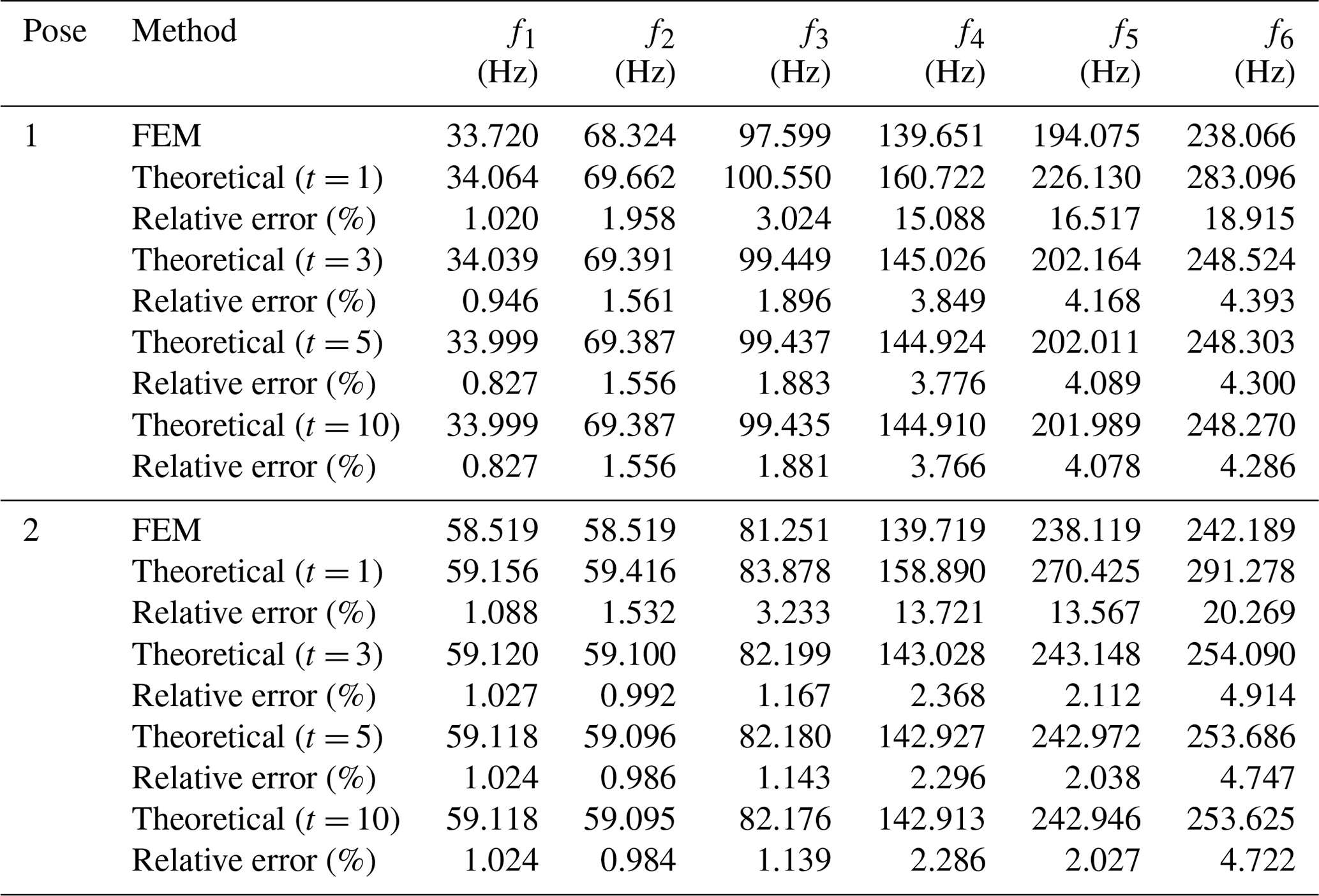
The results for pose 1 in Table 2 show that even when the rods are considered single elements, the relative errors between the natural frequencies obtained by the theoretical method and the FEM for the first, second, and third modes are only 1.020 %, 1.958 %, and 3.024 %, respectively. However, the errors for the fourth, fifth, and sixth modes are as high as 15.088 %, 16.517 %, and 18.915 %, respectively. When the rods are divided into three elements, the errors for the fourth, fifth, and sixth modes rapidly decrease to 3.849 %, 4.168 %, and 4.393 %. Further increasing the number of rod divisions results in no significant reduction in the error. Similar results are obtained for pose 2. The results obtained using the theoretical method are in good agreement with those obtained from the FEM, verifying the acceptability of the proposed theoretical model for natural frequency analysis. The finite element analysis results of the natural frequencies of the 4SRRR parallel robot are shown in Fig. 6.

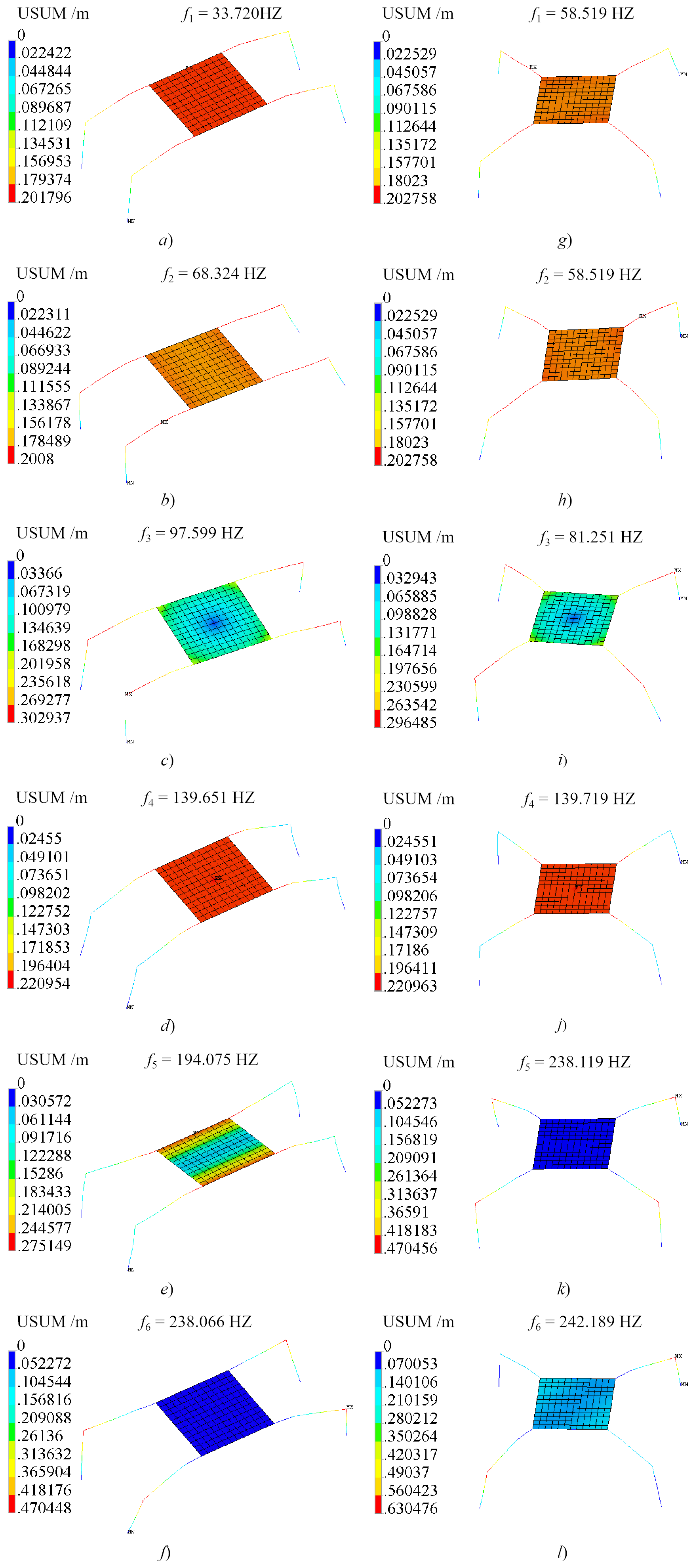
Figure 6 Modal analysis of the 4SRRR parallel robot with the FEM: (a) pose 1: f₁, (b) pose 1: f₂, (c) pose 1: f₃, (d) pose 1: f₄, (e) pose 1: f₅, (f) pose 1: f₆, (g) pose 2: f₁, (h) pose 2: f₂, (i) pose 2: f₃, (j) pose 2: f₄, (k) pose 2: f₅, and (l) pose 2: f₆.

For the two aforementioned postures, when the rods are divided into 10 elements, the comparison of natural frequencies between the theoretical model, subspace iteration method (SIM; Zhang and Lin, 2007), static condensation method (Guyan reduction; Zhang and Lin, 2007), and dynamic condensation method (Kuhar reduction; Zhang and Lin, 2007) is shown in Table 3. The SIM reached the set convergence error (1 %) after just one iteration, and compared to the calculation time of 0.02 s for the exact solution of the theoretical model the SIM reduced the calculation time to 0.005 s, lowering the computational cost by 75 %. The first-order natural frequency of the Guyan reduction matches the exact solution, but there is a significant deviation in the higher-order natural frequencies, making it suitable for scenarios focusing only on the first-order natural frequency. The Kuhar reduction matches the exact solution for the first three natural frequencies but still exhibits considerable errors for higher-order natural frequencies.

Table 3 Comparison of natural frequency between the theoretical method and SIM, Guyan reduction, and Kuhar reduction.

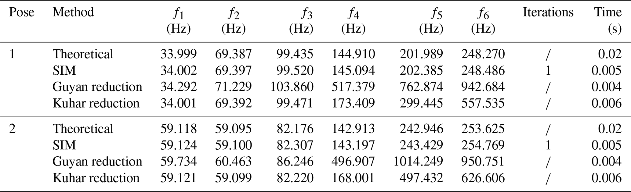
$/$: no iterations required.

In principle, continuous structures have an infinite number of natural frequencies. However, when calculating natural frequencies, we typically discretize the structure into a finite number of modes to solve the problem, with the lowest natural frequency being the fundamental frequency of the structure. It is well known that the fundamental frequency of a structure is very important information. Additionally, the fundamental frequency is related to the structure's vulnerability to resonance failure due to an external frequency load. In other words, if only the fundamental frequency of the mechanism is considered, the accuracy may meet engineering requirements when treating components as single elements. Consequently, the calculation process is significantly simplified, and the dimensions of the overall mass and stiffness matrices are reduced.

Figure 7 presents the MAC (modal assurance criterion) values of the first six modes for the theoretical and finite element solutions of the 4SRRR parallel robot in two typical poses. The diagonal elements in Fig. 7 are all equal to 1, indicating that the theoretical and finite element solutions are approximately identical for the two poses. This is consistent with the results in Table 2, further confirming the accuracy of the theoretical solution. According to Fig. 7a, the mode shape correlation coefficient between the fourth and sixth mode vectors for pose 1 of the quadruped wall-climbing robot is 1, indicating that these two mode vectors are very similar, while all other MAC matrix values are less than 0.12. According to Fig. 7b, the mode shape correlation coefficient between the fifth and sixth mode vectors for pose 2 is 0.62, and the correlation coefficient between the second and fifth mode vectors is 0.52, while all other MAC matrix values are less than 0.34.

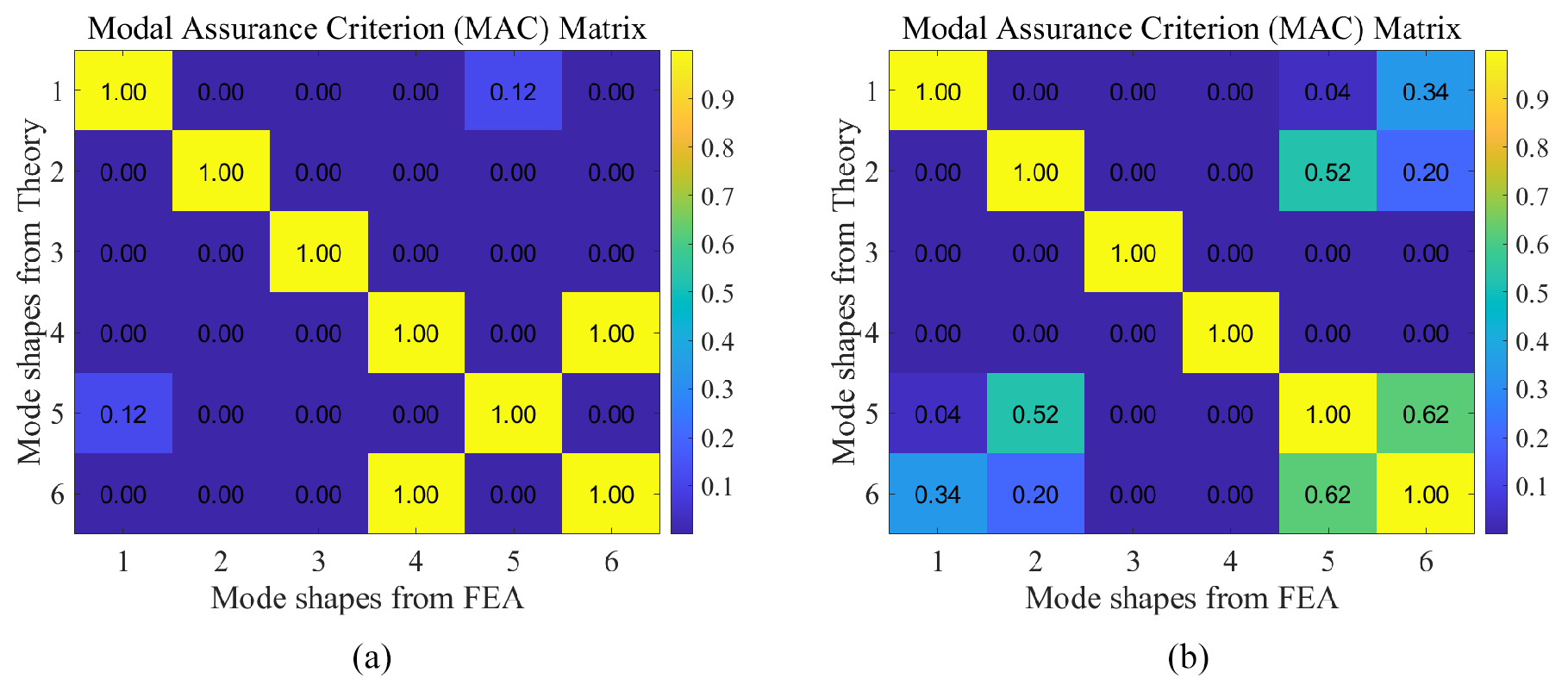
Figure 7 The modal assurance criterion (MAC) values of the modes obtained from the theoretical method and the FEM: (a) pose 1 and (b) pose 2.

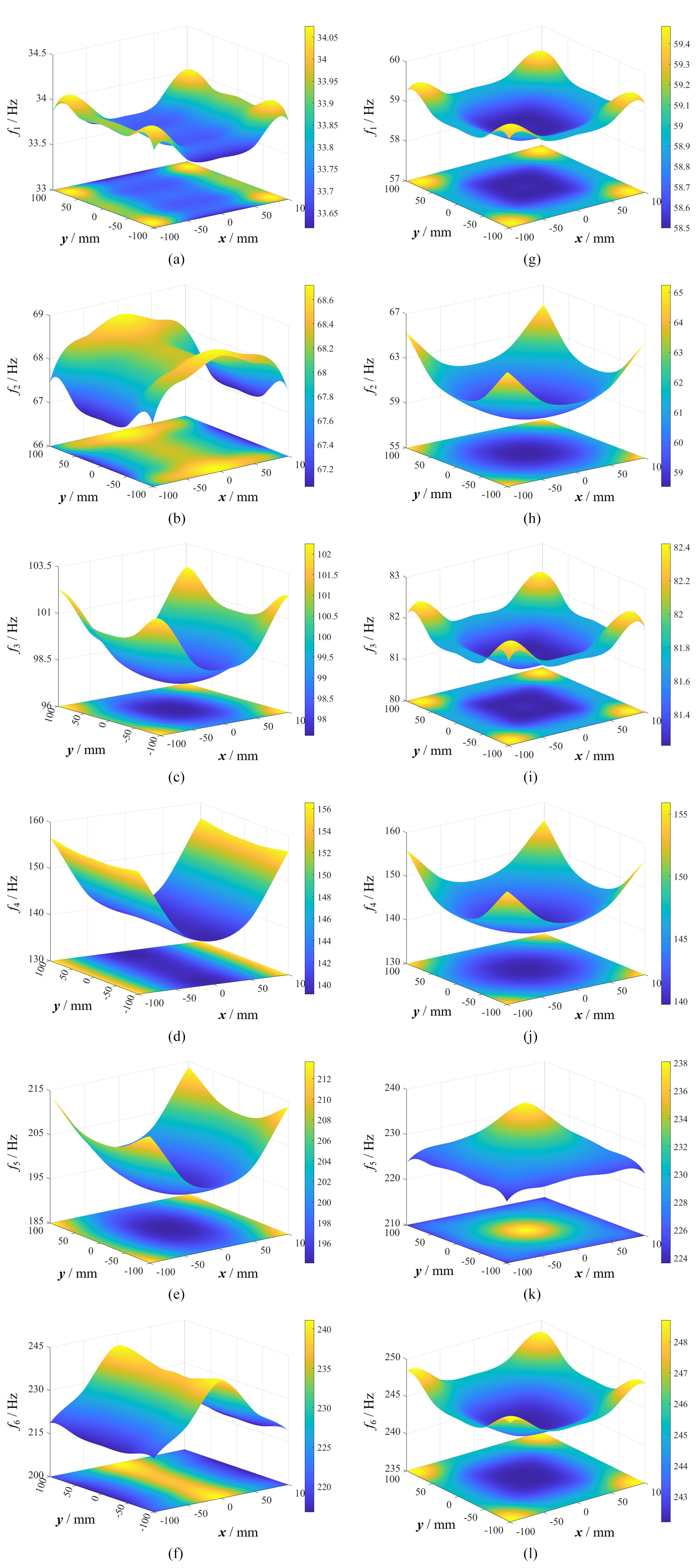
Figure 8 Modal distribution of the 4SRRR parallel robot (pose 1 at z = 0.35, pose 2 at z = 0.40546): (a) pose 1: f₁, (b) pose 1: f₂, (c) pose 1: f₃, (d) pose 1: f₄, (e) pose 1: f₅, (f) pose 1: f₆, (g) pose 2: f₁, (h) pose 2: f₂, (i) pose 2: f₃, (j) pose 2: f₄, (k) pose 2: f₅, and (l) pose 2: f₆.

In the global coordinate system, when the quadruped wall-climbing robot (4SRRR robot) is in pose 1 (pose 2), the geometric center point o of the moving platform moves within the arbitrarily selected working plane z = 0.35 m (z = 0.40546 m) in the range of x = $-\mathrm{0.1}:\mathrm{0.01}:\mathrm{0.1}$, y = $-\mathrm{0.1}:\mathrm{0.01}:\mathrm{0.1}$. Figure 8 shows the distribution of natural frequencies of the 4SRRR robot moving within the plane for pose 1 and pose 2. As shown in Fig. 8, the natural frequencies of the 4SRRR robot in pose 1 and pose 2 are symmetrical about the x axis and y axis, respectively, which is consistent with the structure of the quadruped wall-climbing robot in these poses. Additionally, the natural frequencies of the 4SRRR robot vary in different poses. In engineering, the fundamental frequency, i.e., the first natural frequency, is often of greater concern. A higher fundamental frequency implies a higher control bandwidth, which can reduce the vibration response of the mechanism. Therefore, it is preferable to select the regions with a higher fundamental frequency as the working area. Compared to pose 1, the first natural frequency within the plane of motion in pose 2 is significantly higher, making pose 2 more suitable for on-site operations. Moreover, the first natural frequency in pose 2 has higher values at the four corners of the motion plane.

5 Conclusions

To address the unstructured on-site work requirements in shipyards and large-steel-structure manufacturing plants, this paper develops a 4SRRR quadruped wall-climbing robot. Focusing on the 4SRRR parallel robot, the study first establishes global independent generalized displacement coordinates by combining multipoint constraint elements and linear algebra. Based on these coordinates, the overall mass and stiffness matrices of the robot are constructed, thus obtaining the natural frequencies of the robot. In this research, the moving platform and joints are assumed to be rigid, the spatial elastic deformation of the rods is considered, and Timoshenko beam elements accounting for shear deformation are used to replace Euler–Bernoulli beam elements. The generalized kinetic and potential energies of the elastic deformation of each component are established based on the global independent generalized coordinates. These coordinates encompass the boundary conditions and continuity conditions of the mechanism, having clear physical significance and avoiding the drawbacks of solving a large number of constraint equations simultaneously with the elastodynamic equations.

By comparing the natural frequency calculation results of the theoretical model with those of the finite element model, it is found that even when the rods are considered single elements the error in the first three natural frequencies does not exceed 4 %. When the rods are divided into three elements, the error in the first six natural frequencies does not exceed 4.4 %. Further increasing the number of rod divisions results in no significant reduction in the error. The comparative analysis of the natural frequency calculation results between the theoretical model and the finite element model verifies the correctness of the theoretical model presented in this paper.

In this paper, the joints, actuators, and moving platform are assumed to be rigid, and damping is considered negligible. In future work, the elasticity of the joints, actuators, and moving platform, as well as the damping of the mechanism, will be considered to establish an elastodynamic model that more closely approximates engineering reality, thereby obtaining more accurate results. Additionally, this paper only considers the natural frequency analysis of the 4SRRR quadruped wall-climbing robot. In the future, the combination of the 4SRRR quadruped wall-climbing robot with a 6R welding robotic arm will be considered for natural frequency analysis of the 4SRRR+6R hybrid robot.