Classification of drilling surface roughness on computer numerical control (CNC) machine tools based on Mobilenet_v3_small_improved

Computer numerical control (CNC) machine tool drilling is a crucial process in the contemporary manufacturing sector, facilitating high-precision fabrication of complex components and thus enhancing production efficiency and product quality. Surface roughness serves as a principal quality metric in machining operations. Spindle speed and feed rate are primary determinants influencing the surface roughness during the CNC drilling process. This study introduces data acquisition software developed on the Syntec CNC system and MySQL platform to enable real-time data capture and storage, setting a foundational dataset for subsequent analysis of roughness classification. Additionally, an enhanced roughness classification model using the improved MobileNet_v3_small model is presented. The model integrates dual time–frequency plot features of short-time Fourier transform (STFT) and continuous wavelet transform (CWT) to provide novel input features for the MobileNet_v3_small architecture, the output of which is a workpiece surface roughness classification. Fusing the time–frequency features of STFT and CWT serves to refine the classification capability of the network structure. Validation of the network model followed during training, giving training, validation, and test accuracies of 85.2 %, 84 %, and 85.4 %, respectively. Comparative analysis with other lightweight industrial network models reveals that the improved MobileNet_v3_small model demonstrates average accuracy enhancements of approximately 10 %, 9 %, and 13 % across the training, validation, and test datasets, respectively. Reductions in the root mean square error averaged 0.15. Experimental results indicate the superior classification accuracy of the improved MobileNet_v3_small model in drilling surface roughness.

1 Introduction

Computer numerical control (CNC) machine tool drilling is a prevalent machining technique within the modern manufacturing industry. It finds extensive application across various sectors, including metal processing, automobile manufacturing, aerospace, and electronic equipment production. Within the CNC drilling process, real-time monitoring of processing data assumes a fundamental role in enabling machine condition monitoring and fault diagnosis (Lee et al., 2018; Lauro et al., 2014). The classification of the surface roughness of needed products plays a crucial role in identifying and rectifying defects and issues in the manufacturing process, thereby ensuring product quality and performance while enhancing productivity and competitiveness. Primarily, research on roughness classification serves to enhance the machining precision and surface quality of a workpiece (S. Li et al., 2022; Wang et al., 2023; Otsuki et al., 2022). Through an analysis of the surface roughness characteristics of the drilled surface, we can discern the influence of drilling parameters on surface quality, subsequently optimizing the drilling process parameters to enhance workpiece machining precision and surface quality. Additionally, roughness classification research facilitates fault diagnosis and predictive maintenance in the drilling process. An analysis of surface roughness characteristics enables the identification of potential abnormalities and failures, allowing proactive prevention and maintenance measures. This approach helps prevent equipment damage and production interruptions, leading to improved productivity. Consequently, investigation into CNC drilling surface roughness classification holds significant importance.

Traditionally, roughness measurements have been conducted manually post production, predominantly employing contact and non-contact profilometry methods, which can contribute to decreased factory productivity. To address this challenge, numerous researchers have explored classification and prediction methods for surface roughness based on process parameters (Kim et al., 2024). Research into the classification of surface roughness models primarily includes three key methods: modeling, traditional machine learning, and deep learning. First, Liu et al. (2023) established a theoretical model for surface roughness in ball screw spin milling by considering the combined effects of elastic–plastic deformation and residual height. Song et al. (2022) pioneered the elucidation of the surface roughness formation mechanism during high-speed dry milling of a carbon-fiber-reinforced polymer (CFRP). They developed a precise surface roughness prediction model that incorporates kinematics, dynamics, and carbon fiber distribution. Bhushan (2022) conducted a study focused on investigating the effect of tool wear on surface roughness during the dry turning of composites. They employed a response surface methodology for modeling to predict surface roughness under varying process parameters, including cutting speed, feed, depth of cut, and tip radius.

While the aforementioned studies used a modeling approach to predict and classify surface roughness and yielded some results, they often considered only selected factors that influence the roughness model, resulting in relatively complex and accuracy-limited models. Consequently, some scholars have utilized the correlation between process data and roughness to achieve surface roughness prediction and classification by fitting models through machine learning algorithms. Kong et al. (2020) employed vibration signal features as inputs to a Bayesian linear regression model for roughness prediction. Griffin et al. (2017) investigated the use of acoustic emission as input to a classification tree for predicting surface roughness in micromachining. Liu et al. (2023) introduced a novel method for surface roughness prediction in milling processes, constructing a Bayesian quantile model to obtain predicted roughness and confidence intervals using multisource heterogeneous data, which includes monitoring signals and cutting parameters.

Traditional machine learning methods rely on domain knowledge and manual experience, which may not effectively extract complex features. Thus, Wang et al. (2019) developed a combined convolutional and recurrent deep-learning model to merge spindle power signals with machined surface images, enabling simultaneous tool wear inference and surface roughness prediction. Wu and Lei (2019) utilized features extracted from vibration signals as inputs to a neural network to predict the roughness of routinely machined parts. Abebe and Gopal (2023) investigated the influence of vibration during CNC face-milling machining, exploring constant spindle speed, feed rate, and varying depths of cut in simulation experiments. Surface roughness classification and prediction were achieved by modeling the relationship between vibration and roughness. Deep learning offers advantages such as not requiring manual feature extraction, capturing deep features from raw data, and enhancing model training effectiveness compared to traditional machine learning. Achieving online classification and prediction of workpiece surface roughness necessitates linking machining process data with actual workpiece surface roughness measurements (Moliner-Heredia et al., 2021; Wang et al., 2020; Corne et al., 2017). For metal cutting processes, researchers have employed various methods to predict and classify surface roughness while optimizing machining parameters based on classification results. For instance, prediction models for surface roughness have been established using polynomial models (Parida and Maity, 2019), artificial neural networks (Tian et al., 2022b; Upadhyay et al., 2013; Chen et al., 2017), and Gaussian process machine learning (Liu et al., 2019). These models treat surface roughness as a function of cutting parameters such as cutting speed, feed rate, depth of cut, and vibration, as measured by accelerometers (Chen et al., 2021; Yeganefar et al., 2019; Sekulic et al., 2018). Different process parameter settings result in variations in process characterization data. Consequently, researchers have conducted studies on surface roughness prediction and classification by leveraging diverse process data features during machining, such as sound, vibration, force, and temperature (Tian et al., 2022a; Guleria et al., 2022; Gu et al., 2023).

Due to the variability of CNC machine tools and the diverse types of process data, the effect of different deep-learning network models varies. To establish a direct relationship between process data features and surface roughness as well as an indirect relationship between process parameters and surface roughness, this study proposes a classification model for surface roughness based on process data features under various combinations of process parameters. The CNC drilling roughness classification method presented in this thesis is realized through data acquisition software and a deep-learning algorithm. Initially, a data acquisition system software package is developed using the CNC machine tool implemented on the Visual Studio platform utilizing the C# language, MySQL database, and .NET framework. This software package collects the necessary data for model training. Subsequently, a mapping model between workpiece surface roughness categories and spindle vibration data during the drilling process is established based on the MobileNet_v3_small model. Unlike traditional methods that only rely on a single method to extract time–frequency features for classification or prediction, this thesis introduces a convolutional layer enhancement technique that utilizes short-time Fourier transform (STFT) and continuous wavelet transform (CWT) methods to simultaneously extract the corresponding time–frequency features and perform feature fusion. This approach enhances the time–frequency domain characteristics of the network structure, thus improving classification performance as verified in subsequent network model training.

The innovations presented in this thesis can be summarized as follows:

• 1.

  The data acquisition system software achieves the fusion of acquisition and storage of multisource data from CNC machine tools. It collects, displays, and stores internal CNC machine tool information and external sensor data in real time using a specified format. This foundation is crucial for data analysis and model training.

• 2.

  In data processing, each drilling machining process datum undergoes conversion to time–frequency diagrams based on the STFT and CWT methods. This enables the simultaneous extraction of different time–domain features from the two methods. The feature fusion module is added to the MobileNet_v3_small model to combine the two time–frequency map features to enhance the feature depth extraction and ultimately improve the performance and efficiency of the classification network model.

• 3.

  Considering the complexity of industrial data from multiple sources, the magnitude of the data involved, and the performance of industrial control equipment, experiments are conducted using industrial-grade lightweight network models. The application of these lightweight network models to the surface roughness classification in CNC machine tool drilling has yielded positive results. Furthermore, this lays the groundwork for training models that can perform classification prediction and parameter optimization on industrial control equipment with lower performance.

The remainder of this thesis is structured as follows: Sect. 2 outlines the fundamental process of drilling surface roughness classification. Section 3 details the design and development of the data acquisition system software, including hardware selection in Sect. 3.1 and software interface development in Sect. 3.2. Section 4 covers the data processing process for drilling state data, which facilitates subsequent deep-learning model training. Section 5 introduces the Mobilenet_v3_small_improved roughness classification prediction model, including the dual-feature extraction fusion method for spectrograms and time–frequency graphs in Sect. 5.1 and the lightweight industrial network MobileNet_v3_small model in Sect. 5.2. Section 6 describes the CNC drilling data acquisition experiments and model training, with Sect. 6.1 briefly describing the reasons for choosing vibration signals as sample data. Section 6.2 describes the setup of the experimental bench. Section 6.3 briefly describes the reasons for using spindle speed and feed rate as process parameters for the experiments. Section 6.4 describes the construction of the experimental model. Section 6.5 describes the model training parameter settings.

2 Classification of drilling surface roughness on CNC machine tools based on Mobilenet_v3_small_improved

Figure 1 depicts the flowchart illustrating the classification of surface roughness during CNC machine drilling using Mobilenet_v3_small_improved. The procedural steps entail the collection of three-axis vibration signals from the spindle during CNC drilling and machining, along with measurements of the internal hole diameter and surface roughness at the conclusion of each drilling operation, serving as the primary dataset.

Figure 1 Surface roughness classification flowchart.

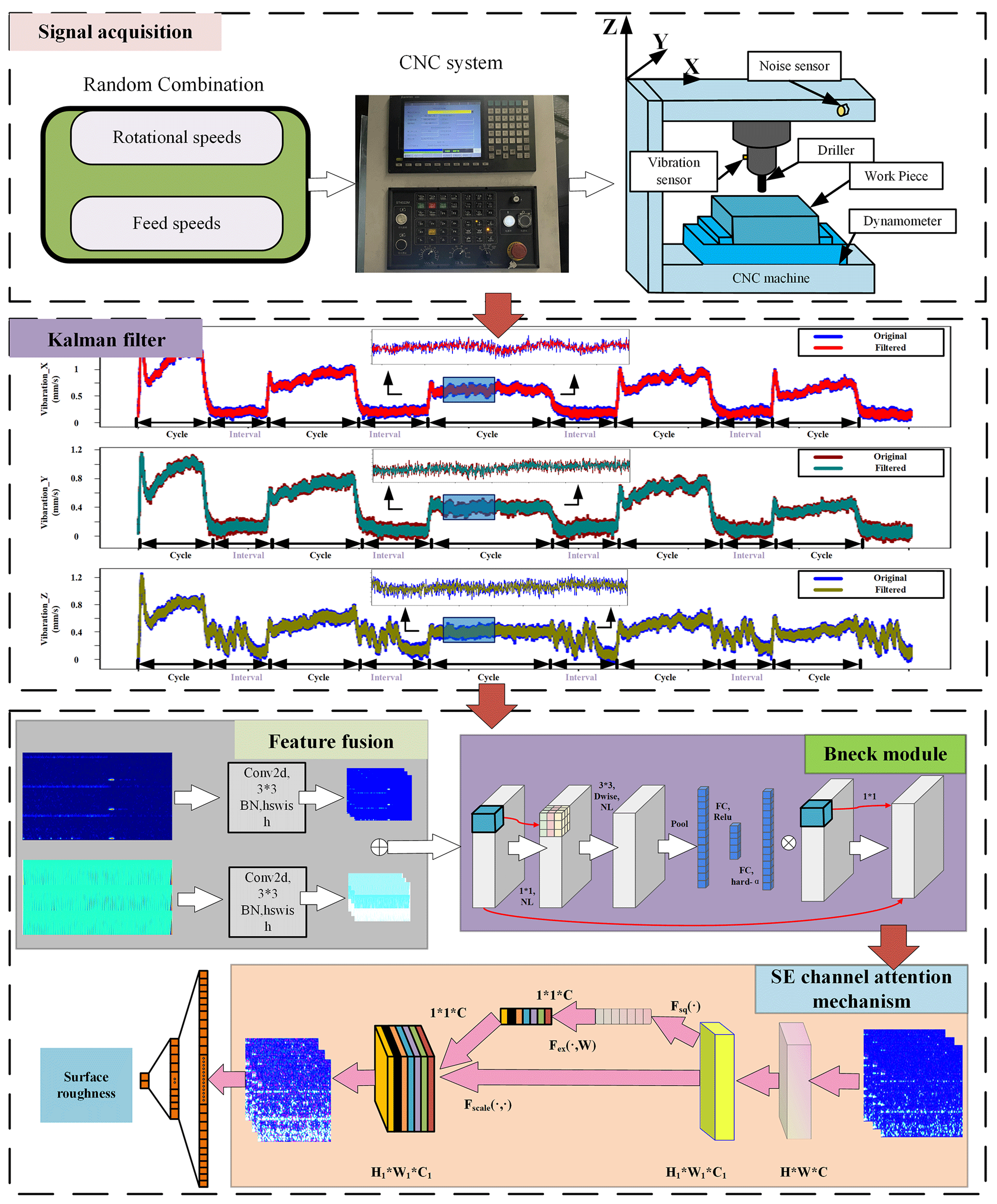
As can be seen in Fig. 1, to commence, the CNC instructions prescribe the machining parameters by employing a random traversal combination of spindle speed and feed rate. Subsequently, during each drilling process, distinct three-axis vibration signals are acquired using four-channel acquisition cards. These signals undergo noise reduction through Kalman filtering. After noise reduction, the three-axis vibration signals undergo transformation into time–frequency diagrams using the STFT and CWT methods. The time–frequency plot features of the two methods are fused as inputs for model training, while the roughness category of the workpiece surface following drilling serves as the output label. Initially, the time–frequency maps obtained using the STFT and CWT methods are processed for convolution and feature extraction, respectively. Subsequently, these two sets of features are amalgamated and input into the network model for training. Leveraging the Mobilenet_v3_small_improved network model structure for training, an indirect mapping model is established for process parameters such as rotational speed, feed rate, and drilling surface roughness. This method facilitates the classification prediction of drilling roughness for varying process parameters (Zhang et al., 2022; Liu et al., 2022; Misaka et al., 2020).

3 CNC drilling data acquisition system development

The development of the CNC drilling data acquisition system includes two essential components: hardware selection and software interface development. The acquisition and processing of process machining data play a pivotal role in the context of deep-learning-based surface roughness classification. The dataset utilized in this study comprises internal information from the CNC machine tool and external sensor data obtained through the in-house-developed data acquisition software.

The internal information sourced from the CNC machine tool includes critical parameters such as spindle speed and spindle feed rate. In contrast, the external sensor data include spindle three-axis vibration measurements, external environmental noise recorded within the machine tool environment, and various electrical parameters (current, voltage, or power) related to the spindle motor output.

3.1 Hardware selection for the data acquisition system

The data acquisition system primarily centers around CNC system MD855 series CNC machine tools. The hardware design includes several key components, including three-axis vibration sensors, noise sensors, voltage transmitters (input), current transmitters (input), voltage transmitters (output), current transmitters (output), a data acquisition card, and a switching power supply. Table 1 provides specific details regarding the sensor parameters and hardware equipment, including the industrial control computer.

Table 1 Hardware device parameters.

$/$: null.​​​​​​​

The three-axis vibration sensor is strategically positioned on the spindle box's side, enabling precise measurement of spindle vibration. Simultaneously, the noise sensor is situated within the machine's outer casing to facilitate monitoring of external environmental noise. Voltage and current transmitters are integrated into the control box located at the CNC machine's back end, allowing for continuous monitoring of voltage and current fluctuations at the spindle's input and output during machining operations. The hardware configuration of the data acquisition system is visually represented in Fig. 2.

Figure 2 Data acquisition system.

3.2 Data acquisition system software interface development

The data acquisition system software utilized in this investigation was crafted using the C# programming language and the .NET framework (Folgado et al., 2023; Adigüzel et al., 2023; Zhang et al., 2023). This software boasts a comprehensive interface, including the primary interface, user management module, data processing module, real-time image rendering module, parameter configuration module, and high-speed drilling acquisition interface module. The holistic architectural representation of the data acquisition software is elucidated in Fig. 3 below.

Figure 3 Data acquisition software architecture.

The communication aspects of the software include Ethernet communication between the industrial control apparatus and the CNC machine tool, serial communication between the industrial control apparatus and the acquisition card, and serial communication between the acquisition card and the sensor. Notably, Ethernet communication between the IPC (Inter Process Communication) and CNC machine tool is achieved through the utilization of the application programming interface (API) function and the TCP (Transmission Control Protocol) network communication protocol. Meanwhile, the serial communications between the industrial control apparatus and the acquisition card and between the acquisition card and the sensor are executed in accordance with the Modbus communication protocol and the serial hardware.

The interaction between the IPC and the CNC machine tool is established by configuring the IP addresses of both the IPC and the CNC machine tool. Additionally, the activation of the core servo functionality of the CNC machine tool facilitates Ethernet communication. Subsequently, the retrieval of internal parameters of the CNC machine tool is achieved through the utilization of the API function. The interface function offers access to a plethora of data, including spindle coordinate information, feed speed, rotational speed, workpiece count, current alarm details, historical alarm records, and tool compensation data.

The MySQL database boasts a rigorously optimized query engine, making it particularly promising in the domain of CNC machine tool data acquisition. This database system excels in swiftly executing queries, even when confronted with substantial data volumes, thus yielding minimal response times. Furthermore, MySQL incorporates a multi-tier security framework, including user authentication, rights management, and data encryption, fortifying the confidentiality and integrity of industrial data. MySQL's compatibility with the standard SQL and open database connectivity interfaces facilitates seamless integration. Consequently, the storage functionality of the data acquisition software is realized well through the utilization of the MySQL database.

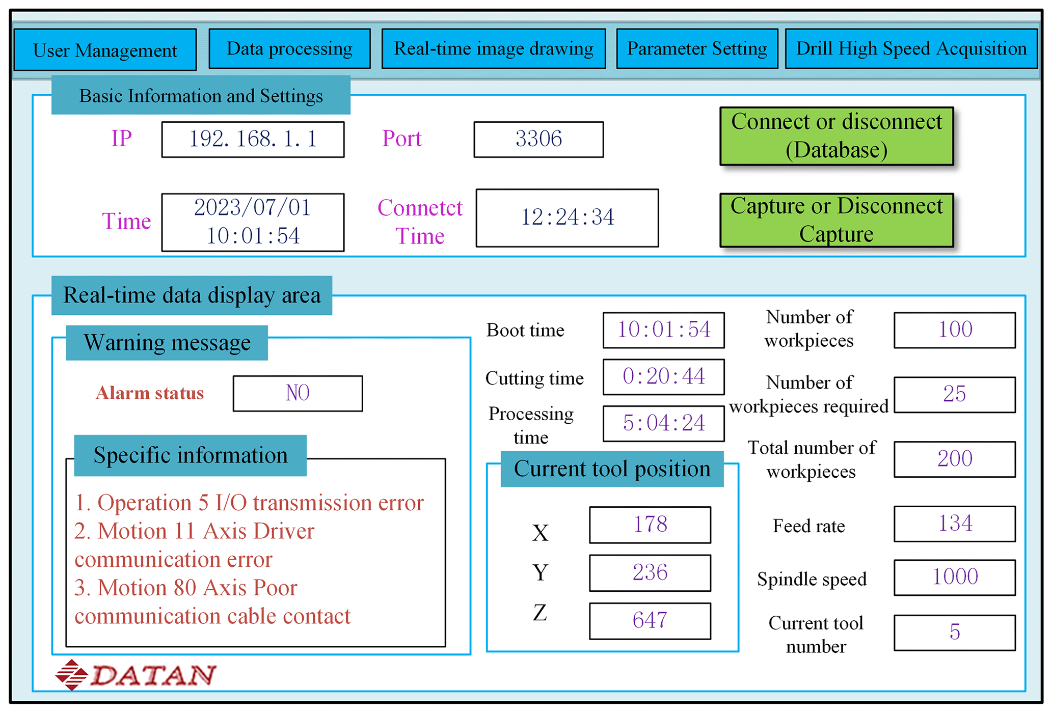
Following the implementation of the aforementioned communication protocols and the establishment of the background machining process database, the internal data from the CNC machine tool and sensor information are systematically stored in the MySQL database, maintaining their inherent format. This experiment culminates in the creation of a data acquisition system rooted in Syntec technology. This system adeptly retrieves real-time internal machine tool information and promptly displays and archives it in real time. The primary interface of the data acquisition software is illustrated in Fig. 4 below.

Figure 4 Main interface of the software.

4 CNC drilling status data processing

The data processing for the CNC drilling status comprises two essential components.

The initial step involves the reduction of noise by Kalman filtering in the raw vibration data, which is subsequently transformed into time–frequency maps using the STFT method.

The second step is the conversion of the raw vibration data to time–frequency maps based on the CWT method (Yao et al., 2023; Y. Li et al., 2022).

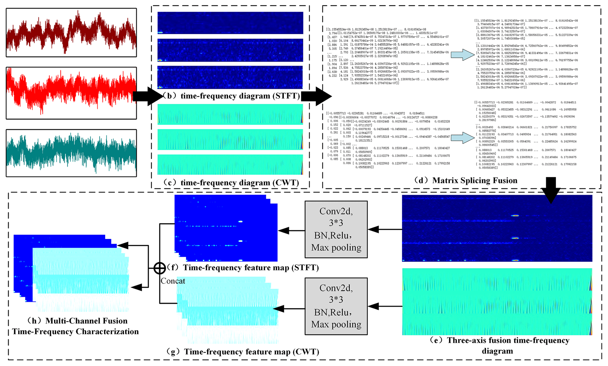
Time–frequency maps provide a visual representation of signal variations across both time and frequency domains. This aids in discerning signal behavior at different time intervals and frequencies, thus facilitating the extraction of time–frequency features pertinent to classification. The process of converting raw data to time–frequency diagrams is elucidated in Fig. 5 below.

The steps for time–frequency plot conversion using the STFT method are as follows:

• 1.

  The STFT method for three-axis vibration data is shown in Eq. (1) below:

  $$\begin{array}{}\text{(1)}& \text{STFT}\left(\mathit{\tau },\mathit{\omega }\right)={\int }_{-\mathrm{\infty }}^{+\mathrm{\infty }}x\left(\mathit{\tau }\right)h(\mathit{\tau }-t)e^{-j\mathit{\omega }\mathit{\tau }}\mathrm{d}\mathit{\tau },\end{array}$$

  where h(τ−t) is the window function. Commonly used window functions include the rectangular window function, the triangular window function, and the Hanning window function.

• 2.

  Plot the STFT time–frequency maps using time as the horizontal coordinate, frequency as the vertical coordinate, and the image color intensity as the magnitude size.

The steps for time–frequency plot conversion using the CWT method are as follows:

• 1.

  Perform a wavelet transform on the three-axis vibration data, as shown in Eq. (2) below:

  $$\begin{array}{}\text{(2)}& W_f(a,b)={\displaystyle \frac{\mathrm{1}}{\sqrt{a}}}{\int }_{-\mathrm{\infty }}^{\mathrm{\infty }}f\left(t\right)\times \mathit{\phi }\times \left({\displaystyle \frac{t-b}{a}}\right)\mathrm{d}t,\end{array}$$

  where W_f(a,b) is a complex function in the time–frequency domain, f(t) is a three-axis vibration data function, φ is a db4 wavelet basis function, the number of wavelet transform layers is six, a is a telescoping parameter, and b is a translational parameter.

• 2.

  Calculate the energy spectrum of a vibration signal at different times and frequencies, as shown in Eq. (3) below:

  $$\begin{array}{}\text{(3)}& E(a,b)=\mathrm{|}W(a,b){\mathrm{|}}^{\mathrm{2}},\end{array}$$

  where E(a,b) is the energy spectrum in the time–frequency domain.

• 3.

  Plot the wavelet time–frequency diagrams by taking time as the horizontal coordinate, frequency $F=\frac{\mathrm{1}}{a}$ as the vertical coordinate, and energy magnitude E(a,b) as the color intensity.

Figure 5 Time–frequency map conversion flowchart.

5 Mobilenet_v3_small_improved roughness classification model

This section includes two primary components.

The STFT–CWT feature fusion methods include the original Mobilenet_v3_small network model. In detail, the feature fusion module is employed to concatenate the features obtained after convolution of STFT–CWT. This integration ensures that the resulting feature map possesses both the time–frequency features of the STFT method and the time–frequency features of the CWT method. Subsequently, the Mobilenet_v3_small architecture is utilized to extract complex features from the feature map post fusion. Through model training, a mapping model between these features and the surface roughness is established.

5.1 STFT–CWT feature fusion methods

The specific flow of STFT–CWT feature fusion is as follows: firstly, the spectral features and time–frequency features of the three-axis vibration signal are extracted based on the STFT and CWT methods and converted to time–frequency maps. Then, the STFT time–frequency map and the CWT time–frequency map are simultaneously input into the convolution module, the corresponding time–frequency map features are extracted through the operations of convolution layer, activation function, and pooling layer; and the features of the time–frequency map are spliced together according to the channel to form the fused feature map. The fused features continue to be input into the Mobilenet_v3_small_improved model to extract complex features fused with different time–frequency map time–domain features and finally classify the surface roughness of the workpiece through the fully connected layer. The STFT–CWT time–frequency feature fusion method is shown in Fig. 6.

Figure 6 STFT–CWT time–frequency feature fusion approach.

It can be seen in Fig. 1 that the feature fusion module is utilized to channel-splice the features of the STFT time–frequency map after convolution and the features of the CWT time–frequency map after convolution, so as to make the feature map have multiple time–frequency features at the same time. The original lightweight network structure of MobileNet_v3_small is used to extract complex features with dual time–domain maps at the same time from the feature map after feature fusion, and the mapping model between the fused features and the surface roughness of the workpiece is established through model training.

5.2 MobileNet_v3_small network model

MobileNet_v3 represents a lightweight neural network architecture tailored to industrial applications. It effectively reduces the hardware requirements of the utilized equipment, presenting promising prospects in practical factory scenarios. Notably, MobileNet_v3_small enhances network performance through the incorporation of two significant technological enhancements: the mobile inverted bottleneck and network slimming. Mobile inverted bottlenecks enrich network expressiveness by introducing learnable activation functions, while network slimming optimizes the network by reducing parameters and computational complexity through sparsity and layer pruning. The network structure of MobileNet_v3_small is shown in Table 2 below.

Table 2 MobileNet_v3_small network structure.

MobileNet_v3_small consists of 3 × 3 and 1 × 1 convolutional layers, 3 × 3 and 5 × 5 bneck layers, a 7 × 7 pooling layer, and a fully connected layer. The primary distinguishing feature within the MobileNet family, as illustrated in Fig. 7, is the utilization of channel-separable convolution, which is pivotal in its lightweight design. This channel-separable convolution can be delineated into two distinct processes:

• 1.

  channel direction channel-separable convolution; and

• 2.

  conventional 1 × 1 convolution generating the designated number of channels.

Figure 7 Channel-separable convolution.

The SE (squeeze-and-excitation) channel attention mechanism, shown in Fig. 8 below, utilizes the FC (filter concatenation) operation implemented by 1 ^∗ 1 convolution, which is essentially the same as FC.

Figure 8 SE channel attention mechanism.

The MobileNet_v3_small model simulates the sigmoid operation using h-sigmoid. Simulate swish using h-swish as shown in Eq. (4). The sigmoid function is simulated using h-sigmoid.

$$\begin{array}{}\text{(4)}& \text{h-swish}\left[x\right]=x{\displaystyle \frac{\text{ReLU6}\left(x+\mathrm{3}\right)}{\mathrm{6}}}\end{array}$$

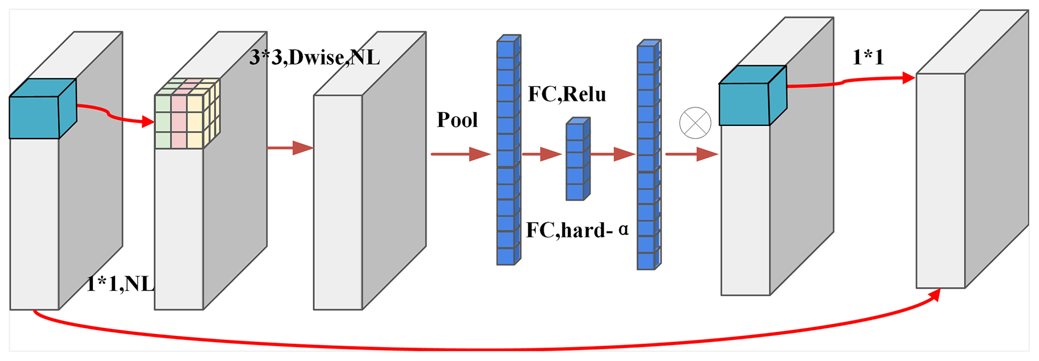
The central module within the MobileNet_v3_small model is the bneck module. This module primarily incorporates channel-separable convolution, the SE channel attention mechanism, and a residual connection. The structural representation of the bneck module is depicted in Fig. 9 below.

Figure 9 The bneck module.

6 CNC drilling data acquisition experiment and model training

6.1 Sample signal selector

Based on modern data acquisition technology, the prediction of surface roughness of parts based on external sensor signals of CNC machine tools has become one of the focus issues of industrial intelligence application. A large number of scientific studies have shown that the effects of different sensor signals applied to different targets and scenes also have differences. The advantages and disadvantages of different sensor signals for surface roughness prediction are shown in Table 3.

Table 3 Advantages and disadvantages of different sensor signals.

Feed is a key process parameter that affects the surface roughness, and it will cause the tool and workpiece contact force to become larger during cutting, which leads to fluctuations in the cutting vibration and directly affects the surface roughness of the workpiece. CNC drilling vibration caused in part by surface ripples fluctuates in the relative displacement between the tool and the workpiece, which in turn leads to the variability of the surface roughness. According to the above formula for surface roughness and the analysis of factors affecting surface roughness, feed, and tip radius, spindle speed is the main factor affecting surface roughness. The above parameter changes will directly cause significant changes in the three-axis vibration data, while the temperature, power, noise, and other signals for the indirect effect exist in the change in high latency, sensitivity, and other weak characteristics. Therefore, this experiment adopts the three-axis vibration signal as the main data sample.

6.2 CNC drilling data acquisition experiment

The experimental setup features a CNC machine tool equipped with the CNC system, model MD855. This platform comprises various components, including a tool magazine, machining platform, drill, cutting fluid system, CNC control system, noise sensor, three-axis vibration sensor, and current and voltage transmitters. A visual representation of the experimental platform can be seen in Fig. 10.

Figure 10 Experimental platform.

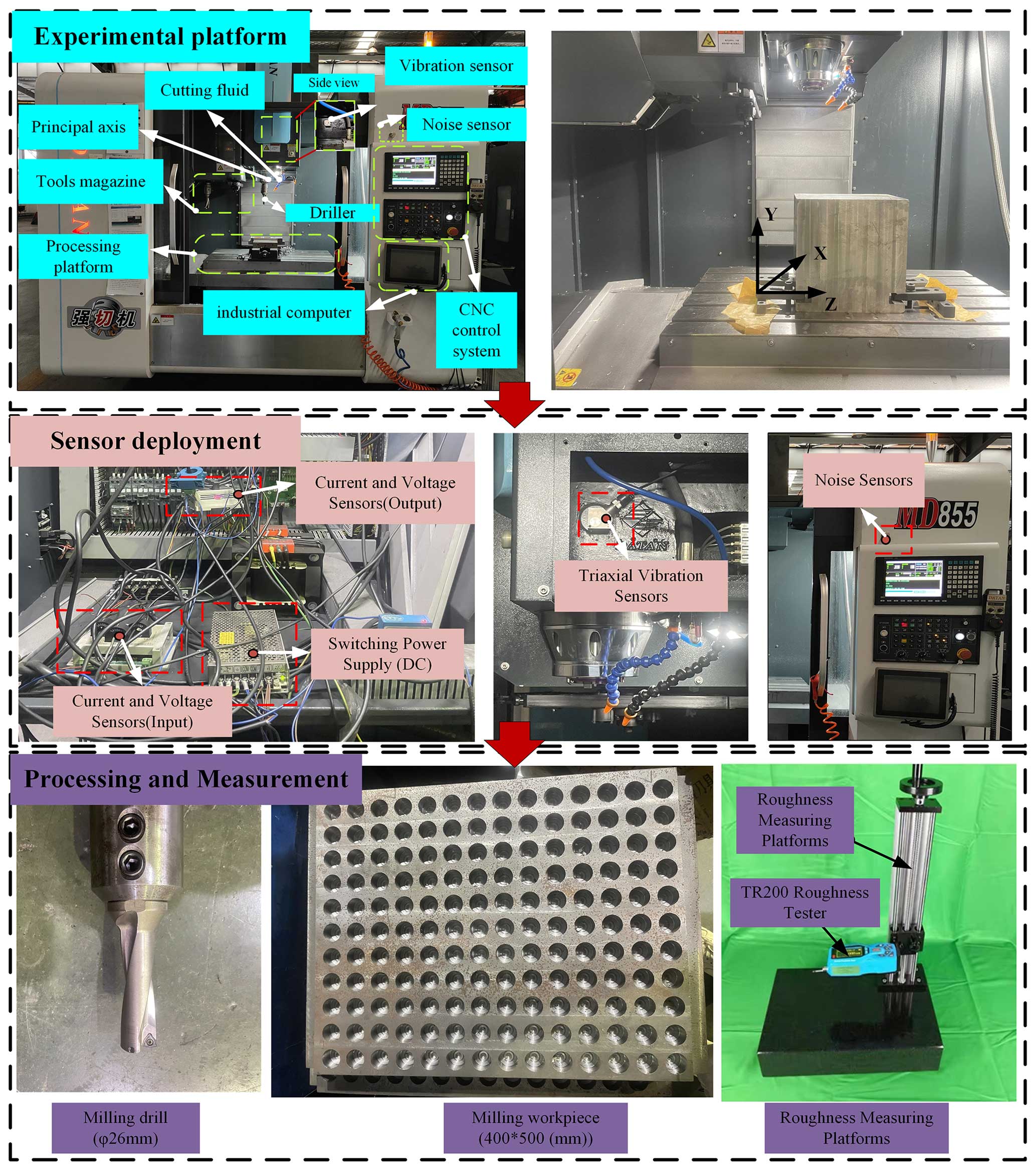
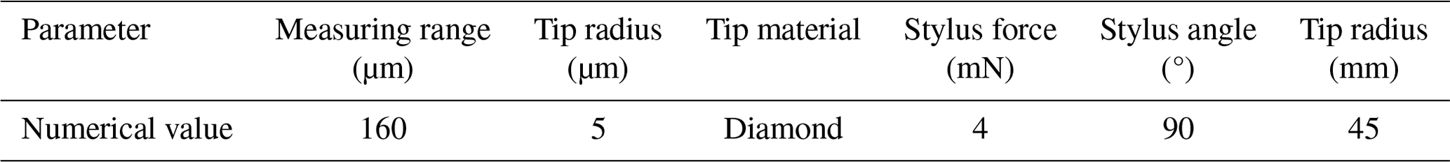
The roughness of the surface of the inner hole of the workpiece after drilling experiments using the TR200 model's portable roughness meter to measure the surface roughness of the workpiece and the roughness-instrument-specific parameters is shown in Table 4. From the table the following can be seen: the roughness instrument's small shape, measuring range, and sampling length to factory workpiece-certified inspection standard Ra1.6. The resolution of 0.001 µm can be a more accurate measurement of the surface roughness value.

Table 4 Parameters of the roughness gauge.

The specific parameters of the roughness measurement sensor equipped with the roughness meter are shown in Table 5, from which it can be seen that the matching sensor of the roughness meter is made of diamond material, the stylus force is 4 mN, and the angle of the stylus is 90°. The radius of the guide head is 45 mm, which can measure the surface roughness of the drilled bore completely.

Table 5 Roughness gauge sensors.

6.3 Analysis of drilling machining parameters

In the current field of CNC drilling processing, there is no specific formula for surface roughness and drilling processing parameters. Feng et al. (2023), based on the spindle speed and feed rate of deep-hole drilling in chip morphology research, had a greater impact on the surface roughness and the chip shape. With reference to the theoretical formulas of surface roughness in turning and milling, according to the influencing factors of surface roughness in drilling machining and the actual machining experience of enterprises, the spindle speed and feed rate are taken as variables to conduct drilling experiments. When the turning depths of the cut and feed are large, the surface roughness of the workpiece is determined by the straight part of the cutting edge, and the surface roughness can be calculated using the following Eq. (5):

$$\begin{array}{}\text{(5)}& R_a={\displaystyle \frac{f}{c\tan k_{\mathrm{r}}+c\tan k_{\mathrm{r}}^{\prime }}},\end{array}$$

where f is the tool feed (mm r⁻¹), k_r and $k_{\mathrm{r}}^{\prime }$ are the primary and secondary deflection angles of the tool, and R_a is the surface roughness value.

The turning depth of the cut and feed is small, the surface roughness of the workpiece is determined by the arc part of the cutting edge, and the surface roughness can be calculated using the following Eq. (6):

$$\begin{array}{}\text{(6)}& R_a=r\left(\mathrm{1}-\cos {\displaystyle \frac{\mathit{\alpha }}{\mathrm{2}}}\right)={\displaystyle \frac{f^{\mathrm{2}}}{\mathrm{8}r}},\end{array}$$

where f is the tool feed (mm r⁻¹), R_a is the surface roughness value, r is the radius of the tool tip arc, and α is the tool center angle.

The theoretical roughness of flat-end milling can be calculated using the following Eqs. (7) and (8) (Eq. 7 for forward milling, Eq. 8 for reverse milling):

$$\begin{array}{}\text{(7)}& {\displaystyle }{R}_a={\displaystyle \frac{f^{\mathrm{2}}}{\mathrm{32}\left(r+\frac{f_n}{\mathit{\pi }}\right)}},\text{(8)}& {\displaystyle }{R}_a={\displaystyle \frac{f^{\mathrm{2}}}{\mathrm{32}\left(r-\frac{f_n}{\mathit{\pi }}\right)}},\end{array}$$

where f is the feed amount per tooth, n is the spindle speed, and r is the radius of the tool tip arc.

According to the above turning and milling roughness theoretical formula, the feed for the two cutting modes in the surface roughness has an important impact on the parameters, and the feed is a part of the feed rate. The size of the feed affects the height of the metal residue on the cutting surface of the workpiece, and a large feed leads to a higher height of the metal residue on the surface and a higher peak height in the R_a roughness calculation, which ultimately affects the surface quality of the workpiece. Therefore, this study uses the feed rate and spindle speed as the control variables for the process parameter combination drilling experiment.

The spindle three-axis vibration data are used in this experiment in Hangzhou, a CNC machine tool company MD855 model three-axis composite machining CNC machine for collection.

• 1.

  Experimental equipment and instruments: MD855 Syntec CNC system three-axis composite machining CNC machine tools, 26 mm diameter U-type drilling, the workpiece material for the 45 Steel, the workpiece size of 400 mm × 500 mm × 50 mm, three-axis vibration sensors, an eight-channel data acquisition card, and an industrial control computer. The vibration sensor is installed in the column on the inner side of the spindle box for collecting the vibration signals generated by the spindle on the x, y, and z axes during the machining process.

• 2.

  Experimental process parameter settings: the spindle speed interval is 1500 to 1900 rpm, the data interval is set to 10 rpm, the number of groups is 40, the feed speed interval is 80 to 170 mm min⁻¹, the data interval is set to 3 mm min⁻¹, and the number of groups is 30. The above parameters were randomly combined to obtain 1200 different combinations of processing parameters. The drilling parameters are shown in Table 6.

Table 6 Machining cutting parameters.

6.4 Model construction

The drilling surface roughness classification prediction model proposed in this paper consists of two parts: (1) the Mobilenet_v3 network model and (2) the multichannel feature-splicing and fusion method based on multiple time–frequency diagrams (STFT and CWT). The specific network model construction process is as follows:

• 1.

  Based on the data acquisition system to collect the three-axis vibration signals of the CNC spindle, the original vibration signals are filtered and processed based on the Kalman filtering method, and the original vibration signals can be expressed by Eq. (9):

  $$\begin{array}{}\text{(9)}& \mathbf{X}=\left\{x_{m,n}\mathrm{}\mathrm{}\mathrm{}\mathrm{}\mathrm{}\mathrm{}\mathrm{}\times x_{m,n}\in R^{\mathit{\alpha }\times \mathit{\beta }}\right\},\end{array}$$

  where X is a matrix of α rows and β columns, m is the matrix row position, n is the matrix column position, α is the number of spindle vibration signals, β is the number of sampling points, and each row of the matrix represents the vibration time series signal.

• 2.

  Construct a discrete linear system model based on the above vibration time series signals. The specific filtering recursive update equation can be calculated using Eqs. (10), (11) and (12):

  $$\begin{array}{}\text{(10)}& {\widehat{x}}_{n,n}=\left(\mathrm{1}-K_n\right){\widehat{x}}_{n,n-\mathrm{1}}+K_n{z}_n,\end{array}$$

  where z_n is the current vibration value (any vibration value in the time series), x_m,n and ${\widehat{x}}_{n,n-\mathrm{1}}$ are the vibration estimates at the previous moment, and ${\widehat{x}}_{n,n}$ is the current optimal vibration estimate.

  $$\begin{array}{}\text{(11)}& p_{n,n}=\left(\mathrm{1}-K_n\right)p_{n,n-\mathrm{1}},\end{array}$$

  where K_n is the Kalman gain, $p_{n,n-\mathrm{1}}$ is the estimated uncertainty calculated during the previous filter estimation, and p_n,n is the uncertainty of the current state estimation.

  $$\begin{array}{}\text{(12)}& K_n={\displaystyle \frac{p_{n,n-\mathrm{1}}}{p_{n,n-\mathrm{1}}+r_n}}\end{array}$$

  In order to simplify the calculation, the system dynamic model of the vibration signal is approximated as a linear constant model in this experiment, so the state extrapolation equation can be calculated using Eq. (13):

  $$\begin{array}{}\text{(13)}& x_{n+\mathrm{1},n}=x_{n,n},\end{array}$$

  where $x_{n+\mathrm{1},n}$ is the predicted value.

  Similarly, the covariance extrapolation equation can be calculated using Eq. (14):

  $$\begin{array}{}\text{(14)}& p_{n+\mathrm{1},n}=p_{n,n},\end{array}$$

  where $p_{n+\mathrm{1},n}$ is the predicted uncertainty.

• 3.

  Based on STFT and CWT, the three-axis vibration signals are converted to uniaxial time–frequency maps T_STFT and T_CWT, respectively. STFT can be calculated using Eq. (15):

  $$\begin{array}{}\text{(15)}& \text{STFT}\left(\mathit{\tau },\mathit{\omega }\right)={\int }_{-\mathrm{\infty }}^{+\mathrm{\infty }}x\left(\mathit{\tau }\right)h\left(\mathit{\tau }-t\right)e^{-j\mathit{\omega }\mathit{\tau }}\mathrm{d}\mathit{\tau }.\end{array}$$

  CWT can be calculated using Eq. (16):

  $$\begin{array}{}\text{(16)}& W_f(a,b)={\displaystyle \frac{\mathrm{1}}{\sqrt{a}}}{\int }_{-\mathrm{\infty }}^{\mathrm{\infty }}f\left(t\right)\times \mathit{\phi }\times \left({\displaystyle \frac{t-b}{a}}\right)\mathrm{d}t.\end{array}$$
• 4.

  The three-axis vibration time–frequency maps are converted to RGB image matrices, and the image matrix conversion can be calculated using Eq. (17):

  $$\begin{array}{}\text{(17)}& S_{m,n}\in R^{\mathit{\alpha }\mathit{\beta }\mathit{\gamma }},\end{array}$$

  where α is the number of pixel points of the image in the width direction, β is the number of pixel points of the image in the height direction, and γ is the number of channels in the image.

• 5.

  The RGB image matrix S_m,n is spliced and merged based on the following Eq. (10) to obtain the fused image matrix T_Rn of the multi-axis vibration signal of each sample, and the matrix T_Rn is converted to an image to obtain the fused time–frequency image of the multi-vibration axial signal AT_Rn. The conversion of the fused time–frequency image can be calculated using Eq. (18):

  $$\begin{array}{}\text{(18)}& T_{\mathrm{Rn}}=\text{connection}\left[T_{\mathrm{0}},T_{\mathrm{1}},T_{\mathrm{2}},\mathrm{\cdots },T_n\right],\end{array}$$

  where “connection” is the matrix splicing operation, T_n is the three-channel matrix of the axial vibration signal, and n is the number of vibration signals.

• 6.

  T_STFT and T_CWT are convolved and normalized by BN layer, Relu activation function, and maximum pooling layer to obtain T_ST and T_CW feature maps, respectively. The multiple time–frequency features are fused based on the Add operation, and the feature fusion method can be calculated using Eqs. (19), (20), and (21):

  $$\begin{array}{}\text{(19)}& {\displaystyle }{T}_{\mathrm{ST}}=\text{Relu}\left\{\text{BN}\left[\text{Conv}\left(T_{\mathrm{FFT}}\right)\right]\right\},\text{(20)}& {\displaystyle }{T}_{\mathrm{CW}}=\text{Relu}\left\{\text{BN}\left[\text{Conv}\left({\text{AT}}_{\mathrm{Rn}}\right)\right]\right\},\text{(21)}& {\displaystyle }{T}_{\mathrm{RT}}=\text{Add}\left[\text{Maxpool}\left(T_{\mathrm{R}\mathrm{1}},T_{\mathrm{R}\mathrm{2}}\right)\right],\end{array}$$

  where Conv is the convolution operation, BN is the normalization operation, Relu is the activation operation, and Maxpool is the maximum pooling operation. The Add operation can be calculated using Eq. (22):

  $$\begin{array}{}\text{(22)}& Z_{\mathrm{Add}}=\sum _{i=\mathrm{1}}^c{X}_i\ast K_i+\sum _{i=\mathrm{1}}^c{Y}_i\ast K_i,\end{array}$$

  where c is the number of channels and ∗ is the convolution operation.

• 7.

  The fused feature maps are fed into the Mobilenet_v3 network model as input; the surface roughness categories are used as output to construct the drilling surface roughness classification prediction model.

  $$\begin{array}{}\text{(23)}& {\text{Output}}_{\mathrm{roughness}}=\text{Model}\left({\text{Input}}_{T_{\mathrm{RT}}}\right),\end{array}$$

  where roughness is the surface roughness category, Model is the Mobilenet_v3 network model, and T_RT is the fused feature map.

6.5 Parameterization

The experiments were programmed using Python as the primary language, with the PyTorch 1.7.0 framework, Cuda 10.1, and an RTX1050Ti graphics card. The chosen optimizer is the Adam optimizer, and the learning rate is dynamically adjusted using the LambdaLR function.

The LambdaLR function adapts the learning rate based on the current epoch value, following a specified lambda function. The adjustment process involves calculating the cosine function value, mapping it to the range of [lrf,1], and ultimately multiplying it by the initial learning rate (lr) to obtain the learning rate for the current epoch. The lr is $\mathrm{1}\times {\mathrm{10}}^{-\mathrm{3}}$, and the lrf is $\mathrm{1}\times {\mathrm{10}}^{-\mathrm{5}}$. Additionally, the input images undergo normalization to 224 × 224, with a batch size set to 16 and the total number of epochs set to 80.

All five models adhere to the same training parameters throughout the training process. This paper focuses on training Mobilenet_v3_small_improved in comparison to other lightweight networks. The specific model training parameters are detailed in Table 7.

Table 7 Model training parameters.

The roughness grade holds significant importance as a classification label for evaluating product quality, controlling manufacturing processes, optimizing product design, and enhancing market competitiveness. Its practical application value extends to both the manufacturing industry and product development.

As a pivotal quality control indicator in the manufacturing process, roughness grade plays a crucial role. By classifying different roughness grades, it becomes possible to assess the stability and consistency of the production line, promptly identify potential issues in the manufacturing process, and make necessary adjustments to enhance product consistency and reliability. In the context of this experiment, the roughness grade for the inner surface of machined holes is categorized into two classes.

Ra0.05–Ra1.6 comprise a total of 844 samples, and Ra1.6–Ra6.3 comprise a total of 356 samples. The calculation of roughness is presented in Eq. (24) below:

$$\begin{array}{}\text{(24)}& R_a={\displaystyle \frac{\mathrm{1}}{l}}{\int }_{\mathrm{0}}^l\mathrm{|}y\mathrm{|}\mathrm{d}x,\end{array}$$

where l is the sampling length and y is the distance from each point to the center line.

The root mean square error (RMSE) loss function plays a pivotal role in assessing the prediction accuracy of the network model during training. In this experiment, RMSE loss and the correctness of the test set classifications serve as key indicators for evaluating the model's performance.

Considering the five model structures described previously, we monitor the correctness and loss values for the training set, validation set, and test set throughout the training process. Additionally, the RMSE loss curve is presented in Fig. 1 below. The calculation of the RMSE is outlined in Eq. (25).

$$\begin{array}{}\text{(25)}& \text{RMSE}=\sqrt{{\displaystyle \frac{\mathrm{1}}{n}}{\sum }_{\mathrm{1}}^n{\left(Y_i-y_i\right)}^{\mathrm{2}}},\end{array}$$

where n is the number of predictions, Y_i is the predicted value, and y_i is the true value.

Based on Fig. 11, Fig. 12, and the data presented in Table 8, a comparative analysis of the training results for various industrial lightweight network models (ResNet, ShuffleNet, Densenet, Mobilenet_v3_small, and Mobilenet_v3_large) was conducted using identical training hyperparameters against the Mobilenet_v3_small_improved network model. Several conclusions can be drawn from this multidimensional comparison:

• 1.

  The Mobilenet_v3_small_improved network model demonstrates superior stability in terms of training accuracy, validation accuracy, and testing accuracy, consistently achieving approximately 85 %. In contrast, other network models exhibit significant fluctuations in accuracy. Notably, the Mobilenet_v3_large model shows a training accuracy of 76.5 % and a testing accuracy of 67 %, with substantial accuracy fluctuations.

• 2.

  The Mobilenet_v3_small_improved network model exhibits faster accuracy convergence, reaching convergence at 50 training steps. Of the other industrial lightweight models, the ShuffleNet network model achieves the fastest accuracy convergence, converging at 60 steps.

• 3.

  The Mobilenet_v3_small_improved network model stands out as the optimal performer across various metrics, including training accuracy, validation accuracy, testing accuracy, training loss, and RMSE. It achieves a training accuracy, validation accuracy, and testing accuracy of 85.2 %, 84 %, and 85.4 %, respectively, with a training loss of 0.43 and an RMSE of 0.61. Among the other network models, the best-trained model is the Mobilenet_v3_small network model, with a training accuracy, validation accuracy, and testing accuracy of 75.1 %, 75 %, and 72 %, respectively, accompanied by a training loss of 0.496 and an RMSE of 0.78.

Table 8 Comparison of model training accuracy. The models in bold are the models proposed in this paper, and the values are the training result data corresponding to the models.

Figure 11 Confusion matrix classification result graph.

Figure 12 Graph of the model training results.

Based on the confusion matrix, a variety of classification index parameters can be calculated to assist in determining the correctness of the model's classification prediction results, e.g., total number of samples, precision, correctness, recall, and F_measure. The confusion matrix is shown schematically below.

The total number of samples (“Total”) is the sum of all samples in the test set, and the total number of samples can be calculated using Eq. (26):

$$\begin{array}{}\text{(26)}& \text{Total}=\text{TP}+\text{FP}+\text{TN}+\text{FN},\end{array}$$

where Total is the total number of samples, TP is true, FP is false positive, TN is true negative, and FN is false negative.

Figure 13 Confusion matrix.

Accuracy characterizes the classification prediction accuracy of the model, i.e., the number correctly identified by the model or the total number of samples, and the accuracy can be calculated using Eq. (27):

$$\begin{array}{}\text{(27)}& \text{Accuracy}={\displaystyle \frac{\left(\text{TP}+\text{TN}\right)}{\text{TP}+\text{FP}+\text{TN}+\text{FN}}}.\end{array}$$

“Precision” indicates the proportion of true classes among the samples predicted by the model to be positive classes, and correctness can be calculated using Eq. (29):

$$\begin{array}{}\text{(28)}& \text{Precision}={\displaystyle \frac{\text{TP}}{\text{TP}+\text{FP}}}.\end{array}$$

“Recall” indicates the ratio of the number of positive class samples correctly predicted by the model to the total number of actual positive class samples, and the recall can be calculated using Eq. (30):

$$\begin{array}{}\text{(29)}& \text{Recall}={\displaystyle \frac{\text{TP}}{\text{TP}+\text{FN}}}.\end{array}$$

F_measure is the reconciled mean of correctness and recall, which is used to balance the concern of correctness and recall in model evaluation. F_measure can be calculated using Eq. (31):

$$\begin{array}{}\text{(30)}& F_{\mathrm{measure}}={\displaystyle \frac{\mathrm{2}\times \text{Precision}\times \text{Recall}}{\text{Precision}+\text{Recall}}}.\end{array}$$

Based on the confusion matrix, a variety of model classification prediction performance evaluation index parameters can be obtained, e.g., precision, recall, correctness, and F_measure. The model evaluation parameters are shown in the following Table 9.

• 1.

  In the results of the comparison experiments of each network model, the Mobilenet_v3_small_improved model has a more obvious superiority in each model evaluation parameter, in which the precision rate, recall rate, correct rate, and F_measure are 85.8 %, 85.7 %, 87.1 %, and 0.864, respectively. Compared with the other models, the evaluation parameters have an improvement of approximately 10 % or more, which indirectly shows the correctness of the Mobilenet_v3_small_improved network model in the application of classification prediction for the drilling dataset.

• 2.

  Among the compared network models, the highest precision and recall are in the Mobilenet_v3_small model, but the highest correctness is in the ResNet model. Of the above two network models, the better F_measure is in the ResNet model. According to the analysis of the above results, it can be seen that performance strengths and weaknesses are not convincing enough when using only the correct rate and recall rate to model classification prediction. Combined with the F_measure index, the overall performance evaluation of the model is more convincing.

• 3.

  According to Table 9, the Mobilenet_v3_small_improved model has better smoothness in the evaluation parameters of each model, and the value fluctuation of each parameter is within 1.5 %; the evaluation parameters of the other network models have greater instability, of which the parameter fluctuation of the Mobilenet_v3_small model reaches about 13 %. The stability of the model in actual engineering application is quite important, and enterprise production application pays more attention to the stable and better performance compared with the unstable and excellent performance.

Table 9 Model evaluation parameters.

7 Conclusion

This paper's primary research content and its associated limitations can be summarized as follows:

• 1.

  Design and development of a multisource data acquisition system, incorporating CNC machine tool internal information data and external sensor data: the software architecture was tailored to actual production needs, with the software interface and MySQL database table structure designed to accommodate multisource data. This component enables real-time monitoring and storage of drilling process data, serving as the foundation for subsequent data analysis and deep-learning model training.

• 2.

  Enhancing the Mobilenet_v3_small network model by incorporating a feature fusion module that fuses different time–domain features of the time–frequency maps of the STFT and CWT methods: this augmentation improves the accuracy of the model's surface roughness classification. Notably, the Mobilenet_v3_small_improved network model exhibits exceptional stability, with training accuracy, validation accuracy, and testing accuracy consistently being approximately 85 %, while other network models experience larger accuracy fluctuations. The Mobilenet_v3_large model, for instance, has a training accuracy of 76.5 % and a testing accuracy of 67 %. The Mobilenet_v3_small_improved network model also demonstrates faster accuracy convergence, reaching convergence at just 50 training steps, outperforming other industrial lightweight models such as ShuffleNet, which converges at 60 steps.

• 3.

  The Mobilenet_v3_small_improved network model outperforms the other models in terms of training accuracy, validation accuracy, testing accuracy, training loss, and RMSE. Specifically, it achieves a training accuracy, validation accuracy, and testing accuracy of 85.2 %, 84 %, and 85.4 %, respectively, with a training loss of 0.43 and an RMSE of 0.61. In comparison, the best-performing model of the others is the Mobilenet_v3_small network model, with a training accuracy, validation accuracy, and testing accuracy of 75.1 %, 75 %, and 72 %, respectively, accompanied by a training loss of 0.496 and an RMSE of 0.78.

• 4.

  The Mobilenet_v3_small_improved network model shows average improvements of 10 % in correctness on the training set, 9 % on the validation set, and 13 % on the test set when compared to the ResNet, ShuffleNet, Densenet, Mobilenet_v3_small, and Mobilenet_v3_large models. Additionally, it reduces the average training loss and RMSE loss by 0.05 and 0.15, respectively.

• 5.

  Acknowledging the significance of the dataset in deep-learning model training, it is important to note that noise can significantly impact the experimental results. In this experiment, only basic noise reduction processing was applied to the dataset. Future studies will explore more advanced noise reduction techniques. Moreover, enhancing the sampling rate by improving the performance of the acquisition equipment is considered for subsequent work. While this experiment primarily used three-axis vibration data as the primary parameter for drilling surface roughness classification, future work may involve combining electrical and vibration signals for more robust model feature extraction, thereby improving correctness and reliability during model training.

• 6.

  Building on the research conducted, the trained model's practical utility will be assessed in actual production settings. By configuring different machining process parameters for drilling, the actual roughness category of the final workpiece will be determined. The machining process data will then be input into the trained model to obtain predicted classification results. These predicted results will be compared with actual measured roughness categories to validate the correctness of the trained model. Additionally, based on the trained network model, it will be possible to deduce appropriate drilling process parameters based on the specific roughness requirements of workpieces in actual production, thus minimizing material waste and enhancing factory production efficiency.