Thermomechanical coupled topology optimization of parameterized lattice structures

This paper presents a topology optimization approach for parameterized lattice structures subjected to thermomechanical coupled loads. The proposed approach aims to minimize the compliance of lattice structures while satisfying volume fraction constraints and accurate temperature constraints. A thermomechanical coupled optimization model containing a heat transfer model and a thermoelastic model is utilized for accurate modeling, and the distribution of the temperature field is related to design variables. Numerical homogenization is employed to calculate the effective properties of parameterized lattices, and polynomial interpolation models are used to replace numerical homogenization methods during optimization iterations to reduce computational costs. The proposed method is demonstrated through examples involving battery packs, L-brackets, and machine tool headstocks. Numerical verification results show that the proposed method significantly reduces the compliance of the designed structures compared to traditional solid designs and precisely meets temperature constraints.

1 Introduction

Many mechanical structures, such as battery packs and turbine blades, operate under both mechanical and thermal loads, necessitating sufficient stiffness, thermal conductivity, and other critical properties (Zheng et al., 2022a; Meng et al., 2022). Lattice structures, known for their exceptional characteristics – including a high stiffness mass ratio, energy absorption capability, and negative thermal expansion coefficient – possess qualities that are well-suited to addressing thermomechanical coupled problems (Banhart and Seeliger, 2008; Zhu et al., 2010; Takezawa et al., 2015). Therefore, thermomechanical coupled topology optimization utilizing lattice structures holds great promise for enhancing structural performance under corresponding working conditions.

Plenty of researchers have studied topology optimization methods for thermomechanical coupled problems. Thurier et al. (2019) developed a two-material topology optimization to enhance the stiffness of designed structures under heat flux boundary conditions and several point loads. Zhu et al. (2019) introduced a temperature-constrained topology optimization to address thermomechanical coupled problems. Kambampati et al. (2020) presented a level set topology optimization technique aimed at minimizing compliance, stress, or mass under combined mechanical and thermal loads. Yang et al. (2022) proposed a topology optimization model to improve the heat dissipation and structural stiffness of cages. However, all of these studies focused solely on optimizing structures with solid materials, overlooking the potential benefits of lattice materials with their exceptional performance characteristics.

Topology optimization for lattice structures needs to address both the microscopic design of lattice unit cells and the distribution of the lattice unit cells in the macro design domain. This approach requires the application of homogenization theory to obtain effective properties of the lattice unit cells (Sivapuram et al., 2016). Homogenization theory has been elaborated on (Bensoussan et al., 2011; Torquato and Haslach Jr., 2002), and topology optimization for lattice structures has been applied successfully (Zhang et al., 2015; Gao et al., 2019; Rodrigues et al., 2002). However, the computational cost of performing numerical homogenization remains high.

Parameterizing lattice unit cells involves defining them with several parameters, which significantly reduces the number of design variables, making the computational cost comparable to that of solid units. Wang et al. (2020) developed a concurrent design method for hierarchical structures with parameterized lattice microstructures, demonstrating excellent effectiveness in verified examples. Imediegwu et al. (2019) presented a framework for the multiscale design of lattices and employed a space of polynomials of the 6th degree to describe the relationship between the lattice parameters and effective properties. White et al. (2019) introduced an accurate method for multiscale topology optimization of elastic structures, employing a Sobolev norm neural network to represent the relation between microstructure parameters and homogenized properties. However, these studies are limited to a single physical field.

Due to the excellent properties of the lattice structure, many researchers have explored their application in thermomechanical coupled topology optimization. Jia et al. (2017) presented a concurrent optimization method under mass and thermal conductivity constraints. Wu et al. (2017) developed a topology optimization scheme with parameterized lattices to obtain lightweight injection molds (Wu et al., 2017). However, both studies overlooked thermoelastic forces, which should not be neglected. Yan et al. (2015) proposed an approach to minimize the compliance of thermoelastic lattice structures under mechanical and thermal loads, yet they did not account for heat conduction. Zhou and Geng (2021) introduced a multiscale and multi-material topology optimization method to improve the heat dissipation and load-bearing capacity of the cellular structures. Zheng et al. (2022b) developed a concurrent topology optimization method for thermoelastic structures with random and interval hybrid uncertainties. Guo et al. (2023) proposed a multiscale concurrent topology optimization method for thermoelastic structures under design-dependent varying temperature fields, and their method had excellent generality and stability. Nevertheless, the above three methods are unable to impose alternative maximum temperature constraints.

This paper presents a topology optimization approach for parameterized lattice structures subjected to mechanical and thermoelastic loads. The proposed method aims to minimize the compliance of lattice structures while adhering to volume fraction constraints and precise temperature constraints. A thermomechanical coupled optimization model, incorporating both heat transfer and thermoelastic models, is employed for accurate modeling. Numerical homogenization and polynomial interpolation schemes are used to obtain the effective properties of the parameterized lattices.

Section 2 details the homogenization method and the polynomial interpolation scheme for parameterized lattice units. Section 3 discusses the optimization model, which includes both the heat transfer and thermoelastic models. The sensitivity analysis and optimization workflow are presented in Sect. 4. Section 5 provides numerical examples, including battery packs, L-brackets, and machine tool headstocks. Conclusions are given in the final section.

2 Homogenization of parameterized lattice unit cells

To reduce the computational cost, parameterized lattice unit cells are used as designed unit cells. As shown in Fig. 1, the parameterized lattice unit cell used in this paper is composed of two equal-width branches. By varying the width of these branches, the cruciform lattice can transition from a completely hollow element to a solid element, enhancing the versatility and performance of structures manufactured with this lattice compared to many other types. Assuming that the size of a lattice unit cell is 1×1, the parameter x represents the width of the horizontal and vertical branches. Lattice unit cells with the uniformly varying parameter x are shown in Fig. 2. To avoid tedious calculation in every iteration, effective macro properties of lattice unit cells with the gradient-varying parameter x are calculated and interpolated with a polynomial function.

Figure 1 Lattice material and lattice unit cells.

Figure 2 Lattice unit cells with different parameters x.

Because of the symmetry of the parameterized lattice unit cells, the effective properties can be written as

$$\begin{array}{}\text{(1)}& D^H=\left[\begin{array}{ccc}{D}_{\mathrm{1}}& D_{\mathrm{2}}& \mathrm{0}\\ D_{\mathrm{2}}& D_{\mathrm{1}}& \mathrm{0}\\ \mathrm{0}& \mathrm{0}& D_{\mathrm{3}}\end{array}\right],\end{array}$$

$$\begin{array}{}\text{(2)}& {\displaystyle }{D}_{\mathrm{T}}^H=\left[\begin{array}{ll}k& \mathrm{0}\\ \mathrm{0}& k\end{array}\right],\text{(3)}& {\displaystyle }{\mathit{\alpha }}^H=\left[\begin{array}{l}\mathit{\alpha }\\ \mathit{\alpha }\\ \mathrm{0}\end{array}\right],\end{array}$$

where D^H is the effective elastic matrix, $D_{\mathrm{T}}^H$ is the effective thermal conductivity matrix, and α^H is the effective thermal expansion vector. $D_{\mathrm{1}},D_{\mathrm{2}},D_{\mathrm{3}},k$ and α are the effective parameters. Aluminum is selected as the base material to construct lattice unit cells in this paper. The effective macro properties are calculated using the homogenization method (Andreassen and Andreasen, 2014). In this approach, the lattice unit cell is discretized into ne finite elements. In this article, ne is set to 250 000 (500×500 finite element mesh) to ensure sufficient calculation accuracy and appropriate calculation time. The effective properties can be obtained with Eqs. (4)–(5). The effective elastic matrix D^H can be calculated as

$$\begin{array}{}\text{(4)}& D^H={\displaystyle \frac{\mathrm{1}}{\left|{\mathrm{\Omega }}^E\right|}}\sum _{j=\mathrm{1}}^{\mathrm{ne}}\underset{{\mathrm{\Omega }}^j}{\int }{\left(I-B{u}_j\right)}^{\mathrm{T}}{D}_{\mathrm{0}}\left(I-B{u}_j\right)\mathrm{d}{\mathrm{\Omega }}^j,\end{array}$$

where $\left|{\mathrm{\Omega }}^E\right|$ is the volume of a lattice unit cell, I is a 3×3 identity matrix, B is the strain–displacement matrix, u_j is the displacement matrix of the micro element j containing three displacement vectors resulting from three different unit strains, and D₀ is the elastic matrix of the base material. The effective thermal conductivity matrix $D_{\mathrm{T}}^H$ can be obtained as

$$\begin{array}{}\text{(5)}& D_{\mathrm{T}}^H={\displaystyle \frac{\mathrm{1}}{\left|{\mathrm{\Omega }}^E\right|}}\sum _{j=\mathrm{1}}^{ne}\underset{{\mathrm{\Omega }}^j}{\int }{\left(I_{\mathrm{T}}-B_{\mathrm{T}}{T}_j\right)}^{\mathrm{T}}{D}_{T\mathrm{0}}\left(I_{\mathrm{T}}-B_{\mathrm{T}}{T}_j\right)\mathrm{d}{\mathrm{\Omega }}^j,\end{array}$$

where I_T is a 2×2 identity matrix, B_T is the gradient of the shape function matrix, T_j is the temperature vector caused by the unit thermal load, and D_T0 is the thermal conductivity matrix of the base material. According to the reference (Deng et al., 2013), the effective thermal expansion vector of a lattice unit cell (α^H) is the same as that of the base material α₀ when the lattice unit cell is composed of a single material.

Lattice unit cells with a uniformly varying parameter x are shown in Fig. 2, the effective properties of which can be calculated using the homogenization method. Then the effective properties of lattice unit cells with other parameters x can be obtained using the interpolation method. In this paper, the commonly used design variable – element density ρ – is selected as the design variable. The density ρ can be expressed explicitly by the parameter x as follows:

$$\begin{array}{}\text{(6)}& \mathit{\rho }=-x^{\mathrm{2}}+\mathrm{2}x.\end{array}$$

The effective properties of lattice unit cells with uniformly varying density ρ (an increase of 0.1 every time from 0.1 to 0.9) are calculated, and the effective properties of lattice unit cells with other densities ρ can be obtained with fourth-order polynomial interpolation as follows:

$$\begin{array}{}\text{(7)}& \mathrm{par}=p_{\mathrm{1}}\times {\mathit{\rho }}^{\mathrm{4}}+p_{\mathrm{2}}\times {\mathit{\rho }}^{\mathrm{3}}+p_{\mathrm{3}}\times {\mathit{\rho }}^{\mathrm{2}}+p_{\mathrm{4}}\times \mathit{\rho }+p_{\mathrm{5}},\end{array}$$

where “par” represents an effective parameter (which can be $D_{\mathrm{1}},D_{\mathrm{2}},D_{\mathrm{3}},k$). p₁–₄ are the interpolation coefficients. The interpolation model corresponding to the solid base material aluminum (used in the design of battery packs and L-brackets) is shown in Fig. 3, and it is found that fourth-order polynomials can fit effective parameters well. If a more accurate fitting model is needed, this can be achieved by increasing the order of the polynomial. In addition, the interpolation model of the base material of the machine tool headstock is similar to that of the battery pack and L-bracket.

Figure 3 Effective properties for different densities ρ.

3 Optimization method

3.1 Heat transfer model

The finite element equation of the steady-state heat conduction for a known heat transfer structure is

$$\begin{array}{}\text{(8)}& K_{\mathrm{T}}T=P,\end{array}$$

where T is the temperature field, P is the thermal load, and K_T is the global heat conduction matrix given by

$$\begin{array}{}\text{(9)}& K_{\mathrm{T}}=\sum _{i=\mathrm{1}}^{\mathrm{NE}}{k}_{\mathrm{T}}^i=\sum _{i=\mathrm{1}}^{\mathrm{NE}}\underset{{\mathrm{\Omega }}^i}{\int }{B}_{\mathrm{T}}^{\mathrm{T}}{D}_{\mathrm{T}i}^H{B}_{\mathrm{T}}\mathrm{d}{\mathrm{\Omega }}^i,\end{array}$$

where $k_{\mathrm{T}}^i$ is the heat conduction matrix of the macro element i, NE is the number of macro elements, $B_{\mathrm{T}}^{\mathrm{T}}$ is the transpose of the gradient of the shape function matrix, and $D_{Ti}^H$ is the effective thermal conductivity matrix of macro element i.

3.2 Thermoelastic model

The thermoelastic force F_th caused by inhomogeneous temperature distribution is given by

$$\begin{array}{}\text{(10)}& F_{\mathrm{th}}=\sum _{i=\mathrm{1}}^{\mathrm{NE}}{F}_{\mathrm{th}}^i=\sum _{i=\mathrm{1}}^{\mathrm{NE}}\underset{{\mathrm{\Omega }}^i}{\int }{B}^{\mathrm{T}}{D}_i^H{\mathit{\epsilon }}_{\mathrm{th}i}\mathrm{d}{\mathrm{\Omega }}^i,\end{array}$$

where $F_{\mathrm{th}}^i$ is the thermoelastic force of the macro element i, $D_i^H$ is the effective elastic matrix of the macro element i, and ϵ_thi is the thermal strain matrix of the macro element i given by

$$\begin{array}{}\text{(11)}& {\mathit{\epsilon }}_{\mathrm{th}i}=\mathrm{\Delta }{T}_i{\mathit{\alpha }}^H,\end{array}$$

where ΔT_i is the temperature change of the macro element i, which can be written as

$$\begin{array}{}\text{(12)}& \mathrm{\Delta }{T}_i=\left(t_{\mathrm{1}}^i+t_{\mathrm{2}}^i+t_{\mathrm{3}}^i+t_{\mathrm{4}}^i\right)/\mathrm{4}-t_{\mathrm{ref}},\end{array}$$

where $t_{\mathrm{1}}^i$, $t_{\mathrm{2}}^i$, $t_{\mathrm{3}}^i$, and $t_{\mathrm{4}}^i$ are the nodal temperature values of a macro element and t_ref is the reference temperature value.

After substituting Eq. (11) into Eq. (10), the thermoelastic force F_th can be written as

$$\begin{array}{}\text{(13)}& F_{\mathrm{th}}=\sum _{i=\mathrm{1}}^{\mathrm{NE}}\underset{{\mathrm{\Omega }}^i}{\int }{B}^{\mathrm{T}}{D}_i^H\mathrm{\Delta }{T}_i{\mathit{\alpha }}^H\mathrm{d}{\mathrm{\Omega }}^i.\end{array}$$

It should be remembered here that Eq. (13) will introduce a calculation error when the temperature gradient within an element is not zero (Guo et al., 2023). However, as with all the numerical examples in this article, the calculation error can be ignored when the temperature gradient within the finite element is small.

The thermoelastic force F_th and the mechanical load F_m constitute the total load, and the following equation is used to compute the displacement field U under mechanical and thermal loads:

$$\begin{array}{}\text{(14)}& KU=F_{\mathrm{m}}+F_{\mathrm{th}},\end{array}$$

where K is the global stiffness matrix given by

$$\begin{array}{}\text{(15)}& K=\sum _{i=\mathrm{1}}^{\mathrm{NE}}{k}_i=\sum _{i=\mathrm{1}}^{\mathrm{NE}}\underset{{\mathrm{\Omega }}^i}{\int }{B}^{\mathrm{T}}{D}_i^{H}B\mathrm{d}{\mathrm{\Omega }}^i,\end{array}$$

and k_i is the stiffness matrix of the macro element i.

3.3 Optimization problem formulation

The optimization model of this study can be written in the following forms:

$$\begin{array}{rl}& \text{Find:}{\mathit{\rho }}_e(e=\mathrm{1},\mathrm{2}\mathrm{\cdots }\mathrm{NE}),\\ & \text{Min:}c=U^{\mathrm{T}}KU=\sum _{e=\mathrm{1}}^{\mathrm{NE}}{u}_e^{\mathrm{T}}{k}_e{u}_e,\\ & \text{s.t.}V=\sum _{e=\mathrm{1}}^{\mathrm{NE}}{\mathit{\rho }}_{e}v\le f{V}_{\mathrm{0}},\\ & KU=F_m+F_{th},\\ & K_{\mathrm{T}}T=P;t_k\le t_k^{*},\\ & \mathrm{0}<{\mathit{\rho }}_{\min }\le {\mathit{\rho }}_e\le \mathrm{1},\end{array}$$

where ρ_e is the design variable of the eth macro element, c is the objective function, u_e is the element displacement vector, V is the volume of the structure, V₀ is the design domain volume, v is the volume of a macro element, f is the occupied volume fraction of the material, t_k is the temperature of the kth node, $t_k^{*}$ is the constrained temperature of the kth node, the constrained nodes are subjected to the same temperature constraints represented by t^* in each example of Sect. 5 for convenience, and ρ_min is a small predetermined value that is set to 0.001 to avoid singularity.

4 Sensitivity analysis and optimization workflow

4.1 Sensitivity analysis

4.1.1 Sensitivity analysis of optimization objectives

Sensitivity information is critical for the optimization solver using the gradient-based algorithm. It can be computed using the adjoint method. The following is the sensitivity of compliance c for the design variable ρ_e, which also has several other completely equal but different forms of expressions (Fang et al., 2022; Ooms et al., 2023; Guo et al., 2023):

$$\begin{array}{}\text{(16)}& \begin{array}{rl}{\displaystyle \frac{\partial c}{\partial {\mathit{\rho }}_e}}& ={\displaystyle \frac{\partial {\mathbf{F}}^{\mathrm{T}}}{\partial {\mathit{\rho }}_e}}\mathbf{U}+{\mathbf{F}}^{\mathrm{T}}{\displaystyle \frac{\partial \mathbf{U}}{\partial {\mathit{\rho }}_e}}={\displaystyle \frac{\partial {\left({\mathbf{F}}_m+{\mathbf{F}}_{\mathrm{th}}\right)}^{\mathrm{T}}}{\partial {\mathit{\rho }}_e}}\mathbf{U}+{\mathbf{U}}^{\mathrm{T}}\mathbf{K}{\displaystyle \frac{\partial \mathbf{U}}{\partial {\mathit{\rho }}_e}}\\ & ={\displaystyle \frac{\partial {\mathbf{F}}_{\mathrm{th}}^{\mathrm{T}}}{\partial {\mathit{\rho }}_e}}\mathbf{U}+{\mathbf{U}}^{\mathrm{T}}\left({\displaystyle \frac{\partial {\mathbf{F}}_{\mathrm{th}}}{\partial {\mathit{\rho }}_e}}-{\displaystyle \frac{\partial \mathbf{K}}{\partial {\mathit{\rho }}_e}}\mathbf{U}\right)=\mathrm{2}{\mathbf{U}}^{\mathrm{T}}{\displaystyle \frac{\partial {\mathbf{F}}_{\mathrm{th}}}{\partial {\mathit{\rho }}_e}}\\ & -{\mathbf{U}}^{\mathrm{T}}{\displaystyle \frac{\partial \mathbf{K}}{\partial {\mathit{\rho }}_e}}\mathbf{U},\end{array}\end{array}$$

where the derivative of F_th with respect to ρ_e can be written as

$$\begin{array}{}\text{(17)}& {\displaystyle \frac{\partial F_{\text{th}}}{\partial {\mathit{\rho }}_e}}=\sum _{i=\mathrm{1}}^{\mathrm{NE}}\underset{{\mathrm{\Omega }}^i}{\int }\left(\mathrm{\Delta }{T}_i{B}^{\mathrm{T}}{\displaystyle \frac{\partial D_i^H}{\partial {\mathit{\rho }}_e}}+{\displaystyle \frac{\partial \mathrm{\Delta }{T}_i}{\partial {\mathit{\rho }}_e}}{B}^{\mathrm{T}}{D}_i^H\right){\mathit{\alpha }}^H\mathrm{d}{\mathrm{\Omega }}^i,\end{array}$$

and the derivative of K with respect to ρ_e is

$$\begin{array}{}\text{(18)}& {\displaystyle \frac{\partial K}{\partial {\mathit{\rho }}_e}}=\sum _{i=\mathrm{1}}^{\mathrm{NE}}{\displaystyle \frac{\partial k_i}{\partial {\mathit{\rho }}_e}}=\sum _{i=\mathrm{1}}^{\mathrm{NE}}\underset{{\mathrm{\Omega }}^i}{\int }{B}^{\mathrm{T}}{\displaystyle \frac{\partial D_i^H}{\partial {\mathit{\rho }}_e}}B\mathrm{d}{\mathrm{\Omega }}^i.\end{array}$$

The derivative of $D_i^H$ with respect to ρ_e can be written as

$$\begin{array}{}\text{(19)}& {\displaystyle \frac{\partial D_i^H}{\partial {\mathit{\rho }}_e}}=\left[\begin{array}{ccc}\frac{\partial D_{\mathrm{1}}}{\partial {\mathit{\rho }}_e}& \frac{\partial D_{\mathrm{2}}}{\partial {\mathit{\rho }}_e}& \mathrm{0}\\ \frac{\partial D_{\mathrm{2}}}{\partial {\mathit{\rho }}_e}& \frac{\partial D_{\mathrm{1}}}{\partial {\mathit{\rho }}_e}& \mathrm{0}\\ \mathrm{0}& \mathrm{0}& \frac{\partial D_{\mathrm{3}}}{\partial {\mathit{\rho }}_e}.\end{array}\right]\end{array}$$

The derivative of ΔT_i with respect to ρ_e can be written as

$$\begin{array}{}\text{(20)}& {\displaystyle \frac{\partial \left(\mathrm{\Delta }{T}_i\right)}{\partial {\mathit{\rho }}_e}}=\left({\displaystyle \frac{\partial t_{\mathrm{1}}^i}{\partial {\mathit{\rho }}_e}}+{\displaystyle \frac{\partial t_{\mathrm{2}}^i}{\partial {\mathit{\rho }}_e}}+{\displaystyle \frac{\partial t_{\mathrm{3}}^i}{\partial {\mathit{\rho }}_e}}+{\displaystyle \frac{\partial t_{\mathrm{4}}^i}{\partial {\mathit{\rho }}_{\mathrm{e}}}}\right)/\mathrm{4}.\end{array}$$

4.1.2 Sensitivity analysis of constraints

The temperature of the kth node t_k can be obtained by multiplying the temperature vector by the transpose matrix $\left(P_k^{\mathrm{T}}\right)$ of the unit virtual heat load vector P_k. The kth component of $P_k^{\mathrm{T}}$ is unity, while all the other components are zero (Zhu et al., 2019; Zuo and Xie, 2014).

$$\begin{array}{}\text{(21)}& t_k=P_k^{\mathrm{T}}T\end{array}$$

$$\begin{array}{}\text{(22)}& P_k^{\mathrm{T}}=\mathit{\{}\mathrm{0},\mathrm{0},\mathrm{\dots },\mathrm{1},\mathrm{0},\mathrm{\dots }\mathit{\}}=\left\{p_{\mathrm{1}},p_{\mathrm{2}},\mathrm{\dots },p_k,p_{k+\mathrm{1}},\mathrm{\dots }\right\}\end{array}$$

The sensitivity of t_k for the variable ρ_e is

$$\begin{array}{}\text{(23)}& {\displaystyle \frac{\partial t_k}{\partial {\mathit{\rho }}_e}}=-{\left(T_k\right)}^{\mathrm{T}}{\displaystyle \frac{\partial K_{\mathrm{T}}}{\partial {\mathit{\rho }}_e}}T,\end{array}$$

where T_k is the temperature vector under unit virtual heat load P_k given by

$$\begin{array}{}\text{(24)}& T_k=K_{\mathrm{T}}^{-\mathrm{1}}{P}_k.\end{array}$$

The derivative of K_T with respect to ρ_e can be written as

$$\begin{array}{}\text{(25)}& {\displaystyle \frac{\partial K_{\mathrm{T}}}{\partial {\mathit{\rho }}_e}}=\sum _{i=\mathrm{1}}^{\mathrm{NE}}\underset{{\mathrm{\Omega }}^i}{\int }{B}_{\mathrm{T}}^{\mathrm{T}}{\displaystyle \frac{\partial D_{Ti}^H}{\partial {\mathit{\rho }}_e}}{B}_{\mathrm{T}}\mathrm{d}{\mathrm{\Omega }}^i.\end{array}$$

The derivative of $D_{Ti}^H$ with respect to ρ_e can be written as

$$\begin{array}{}\text{(26)}& {\displaystyle \frac{\partial D_{Ti}^H}{\partial {\mathit{\rho }}_e}}=\left[\begin{array}{cc}\frac{\partial k}{\partial {\mathit{\rho }}_e}& \mathrm{0}\\ \mathrm{0}& \frac{\partial k}{\partial {\mathit{\rho }}_e}\end{array}\right].\end{array}$$

4.1.3 Sensitivity filtering

Sensitivity filtering is used to solve checkerboards and mesh-dependence problems. The sensitivity is modified as follows (Sigmund, 2007):

$$\begin{array}{}\text{(27)}& {\displaystyle \frac{\stackrel{\mathrm{̃}}{\partial c}}{\partial {\mathit{\rho }}_e}}={\displaystyle \frac{{\sum }_{i\in N_e}w\left({\mathbf{x}}_i\right){\mathit{\rho }}_i\frac{\partial c}{\partial {\mathit{\rho }}_i}}{{\mathit{\rho }}_e{\sum }_{i\in N_e}w\left({\mathbf{x}}_i\right)}},\end{array}$$

where N_e is the neighborhood of element e and consists of elements whose center distance from element e is less than the filter radius R, i.e.,

$$\begin{array}{}\text{(28)}& N_e=\left\{i\Vert \Vert {\mathbf{x}}_i-{\mathbf{x}}_e\Vert \le R\right\},\end{array}$$

where x_i is the location of element i. The weighting function w(x_i) is written as

$$\begin{array}{}\text{(29)}& w\left({\mathbf{x}}_i\right)=R-∥{\mathbf{x}}_i-{\mathbf{x}}_e∥.\end{array}$$

4.2 Optimization workflow

The proposed thermomechanical coupled topology optimization problem is solved using the Method of Moving Asymptotes (MMA) optimizer (Svanberg, 1987). The flowchart for the proposed method is shown in Fig. 4. The working steps are outlined below:

•  

  Step 1. Initialize the design variables, boundary conditions, and constraints.

•  

  Step 2. Calculate the effective properties of the lattice unit cells with gradient-varying parameters using Eqs. (4)–(5) and establish the corresponding interpolation function with Eq. (7).

•  

  Step 3. Calculate the effective properties of all macro elements of the designed structure according to the interpolation function (Eq. 7).

•  

  Step 4. Solve the temperature field T and displacement field U with Eqs. (8) and (14).

•  

  Step 5. Calculate the objective and constraint functions.

•  

  Step 6. Analyze and filter the sensitivity.

•  

  Step 7. Update the design variables with the MMA optimizer.

•  

  Step 8. If the iterative convergence criterion is satisfied, stop the iteration and output the optimal topology; otherwise, perform step 9.

•  

  Step 9. Update the design and then go to step 3.

Figure 4 Flowchart for thermomechanical coupled topology optimization.

5 Numerical examples

5.1 Battery pack design

The first example involves designing a battery pack, as depicted in Fig. 5. The load and boundary conditions in this example are similar to those used in the battery pack example by Kambampati et al. (2020), facilitating easier comparison between our method and solid-structure topology optimization methods. The optimized structure designed using our method demonstrates superior performance. The four corners of the battery pack are fixed, and a uniform mechanical load is applied around the battery pack. The temperature surrounding the battery pack remains constant, and 25 batteries are distributed evenly within the pack.

Figure 5 A schematic of a battery pack subject to mechanical and thermal loads.

The design aims to minimize the compliance of the battery pack under volume and temperature constraints. The dimension of the considered battery pack is $\mathrm{0.2}\mathrm{m}\times \mathrm{0.2}\mathrm{m}\times \mathrm{0.05}\mathrm{m}$. All the batteries have a diameter of 2 cm. One-fourth of the battery pack is designed because of its symmetry, and the four-node planar finite element mesh of size 25×25 elements is used. The uniform mechanical load around the battery pack is 10⁷ N m⁻¹. All batteries cannot be designed, and they generate a thermal load of 100 W in their center. The temperature around the battery pack is constant at 0 °C. Young's modulus of the solid base material is 69 GPa, and Poisson’s ratio is 0.3. The thermal conductivity and the thermal expansion coefficient of the solid base material are 235 W m⁻¹ °C⁻¹ and $\mathrm{2.32}\times {\mathrm{10}}^{-\mathrm{5}}$ °C⁻¹. The reference temperature used is 0 °C. The radius of the sensitivity filter is 2.1 finite elements. All the temperature constraints are set in the center of the batteries.

Figure 6 Optimal topologies, their partial enlargement, and the temperature distributions subject to a volume fraction constraint of 40 % and different temperature constraints.

5.1.1 Comparison of different temperature constraints

In this section, the compliance of a battery pack is minimized subject to a volume fraction constraint of 40 % and different temperature constraints of 30, 35, and 40 °C. The optimal topologies, their partial enlargement, and the temperature distributions are shown in Fig. 6. The optimal topologies have been filled with the aforementioned parameterized lattices according to the optimized density, and the middle areas of the optimal topologies have been enlarged for better display. In Fig. 6a, it can be seen that the maximum temperature occurs in the middle because of the distance farther away from the boundary of the constant temperature. Since the battery in the center is farthest from the boundary, most of the lattice unit cells are distributed on the shortest path between it and the boundary, i.e., near their four perpendiculars. In addition, the batteries in the corners are near the boundary, so fewer lattice unit cells are distributed around them to limit the temperature of the batteries.

In Fig. 6b and c, it can be seen that, for the increasing value of the temperature constraint, the lattice unit cells are redistributed to a larger area to minimize compliance under the corresponding temperature constraint. As a result, the compliance of the battery pack is decreased, with the compliance being 5964 and 5213 for the temperature constraints of 35 and 40 °C, respectively. Clearly, it can be found that temperature constraints that are too strict will significantly increase the compliance of the designed structure.

5.1.2 Comparison of different volume fraction constraints

In this section, the compliance of a battery pack is minimized subject to the same temperature constraints of 30 °C and different volume fraction constraints of 50 %, 55 %, and 60 %. Optimal topologies and the corresponding temperature distributions obtained by the proposed approach are shown in Fig. 7. The maximum temperature constraints are satisfied under different volume fraction constraints. As the volume fraction constraint decreases from 60 % to 50 %, the range that the lattices cover decreases and the compliance of the battery pack increases from 3370 to 4996, which reveals a great influence of the volume fraction constraints on the compliance. Interestingly, the temperature distribution of the optimal structure of the battery pack obtained under different temperature constraints is extremely similar. In Fig. 7a, it can be observed that, when there are few materials, large hollow areas appear near the corners with low temperatures.

Figure 7 Optimal topologies and the corresponding temperature distributions subject to a temperature constraint of 30 °C and different volume fraction constraints.

5.1.3 Comparison with solid structures

To illustrate the superior performance of the battery pack obtained using the proposed method, the optimal topology of the battery pack obtained using the proposed method is compared with solid-structure topology optimization. Their objective functions, constraints, and discretizations are the same. The volume fraction and temperature constraint are set to 70 % and 25 °C, respectively. The optimal topology and the corresponding temperature distribution of the battery pack obtained using the solid-structure topology optimization and the proposed method are shown in Fig. 8. The compliance of the battery pack obtained using the proposed method is 3101, which is 18.8 % lower than that of the solid optimal topology, while their corresponding temperature distributions are similar.

Figure 8 Optimal topologies and the corresponding temperature distributions subject to a volume fraction constraint of 70 % and a temperature constraint of 25 °C.

5.2 L-bracket design

The second example designs an L-bracket as illustrated in Fig. 9. The upper end of the L-bracket is fixed, and the L-bracket is subjected to a uniform mechanical load all around except for the upper part. The temperature around the L-bracket is kept constant, and the seven batteries are distributed evenly in the L-bracket.

Figure 9 A schematic of an L-bracket subject to mechanical and thermal loads.

Figure 10 Optimal topologies and the corresponding temperature distributions subject to a volume fraction constraint of 40 % and different temperature constraints.

The design aim of the L-bracket is the same as that of the battery pack. The dimension of the considered L-bracket is $\mathrm{0.2}\mathrm{m}\times \mathrm{0.2}\mathrm{m}\times \mathrm{0.05}\mathrm{m}$, and a $\mathrm{0.06}\mathrm{m}\times \mathrm{0.06}\mathrm{m}\times \mathrm{0.05}\mathrm{m}$ area is removed to model the L-bracket. All the batteries have a diameter of 2 cm. The entire domain is discretized into 50×50 four-node planar finite elements. The uniform mechanical load is 1.25×10⁷ N m⁻¹. All batteries cannot be designed, and they generate a thermal load of 300 W in their center. The temperature of the L-bracket boundary is constant at 0 °C. Young's modulus of the solid base material is 69 GPa, and Poisson's ratio is 0.3. The thermal conductivity and the thermal expansion coefficient of the solid base material are 235 W m⁻¹ °C⁻¹ and $\mathrm{2.32}\times {\mathrm{10}}^{-\mathrm{5}}$ °C⁻¹. The reference temperature used is 0 °C. The radius of the sensitivity filter is 2.1 finite elements. All the temperature constraints are set in the centers of the batteries.

5.2.1 Comparison of different temperature constraints

In this section, the compliance of the L-bracket is minimized subject to a volume fraction constraint of 40 % and different temperature constraints of 35, 40, and 45 °C. The optimal topologies and the corresponding temperature distribution are shown in Fig. 10. With the enhancement of the temperature constraints, there are more and more materials between the battery and the boundary. The color bars of the three temperature field distribution pictures in Fig. 10 are different. If the three temperature graphs are enlarged, it will be found that, although their temperature distributions are similar, their maximum temperatures are 35, 40, and 45 °C, respectively. In order to achieve the most efficient cooling, materials are gathered on the shortest path between the battery and the boundary when the temperature constraint is strong. As a result, the compliance of the L-bracket increases from 7485 to 9928, with the temperature constraint changing from 45 to 35 °C.

5.2.2 Comparison of different volume fraction constraints

In this section, the compliance of the L-bracket is minimized subject to the same temperature constraint of 35 °C and different volume fraction constraints of 50 %, 55 %, and 60 %, respectively. Optimal topologies and the corresponding temperature distributions obtained using the proposed approach are shown in Fig. 11. The maximum temperature constraints are satisfied under different volume fraction constraints. As the volume fraction constraint decreases from 60 % to 50 %, the compliance of the L-bracket increases from 4959 to 6373, which shows the huge effect of volume fraction constraints on compliance.

Figure 11 Optimal topologies and the corresponding temperature distributions subject to a temperature constraint of 35 °C and different volume fraction constraints.

5.2.3 Comparison with solid structures

To display the excellent performance of the L-bracket obtained using the presented approach, the optimal topology of the L-bracket obtained using the proposed method is compared with that obtained using the solid-structure topology optimization method. Their objective functions, constraints, and discretizations are the same. The volume fraction and temperature constraint are set to 70 % and 30 °C, respectively. The optimal topology and the corresponding temperature distribution of the L-bracket obtained using the solid-structure topology optimization and the proposed method are shown in Fig. 12. The compliance of the L-bracket obtained using the proposed method is 4109, which is 20.7 % lower than that of the solid optimal topology, while their corresponding temperature distributions are similar.

Figure 12 Optimal topologies and the corresponding temperature distributions subject to a volume fraction constraint of 70 % and a temperature constraint of 30 °C.

5.3 Machine tool headstock design

The last example designs a machine tool headstock as illustrated in Fig. 13. The middle of the left side of the headstock is fixed. The headstock contains two holes in which the motor (left) and the spindle (right) are located. The headstock is subject to two point loads. The temperature around the headstock is kept constant at 0 °C.

Figure 13 A schematic of a machine tool headstock subject to mechanical and thermal loads.

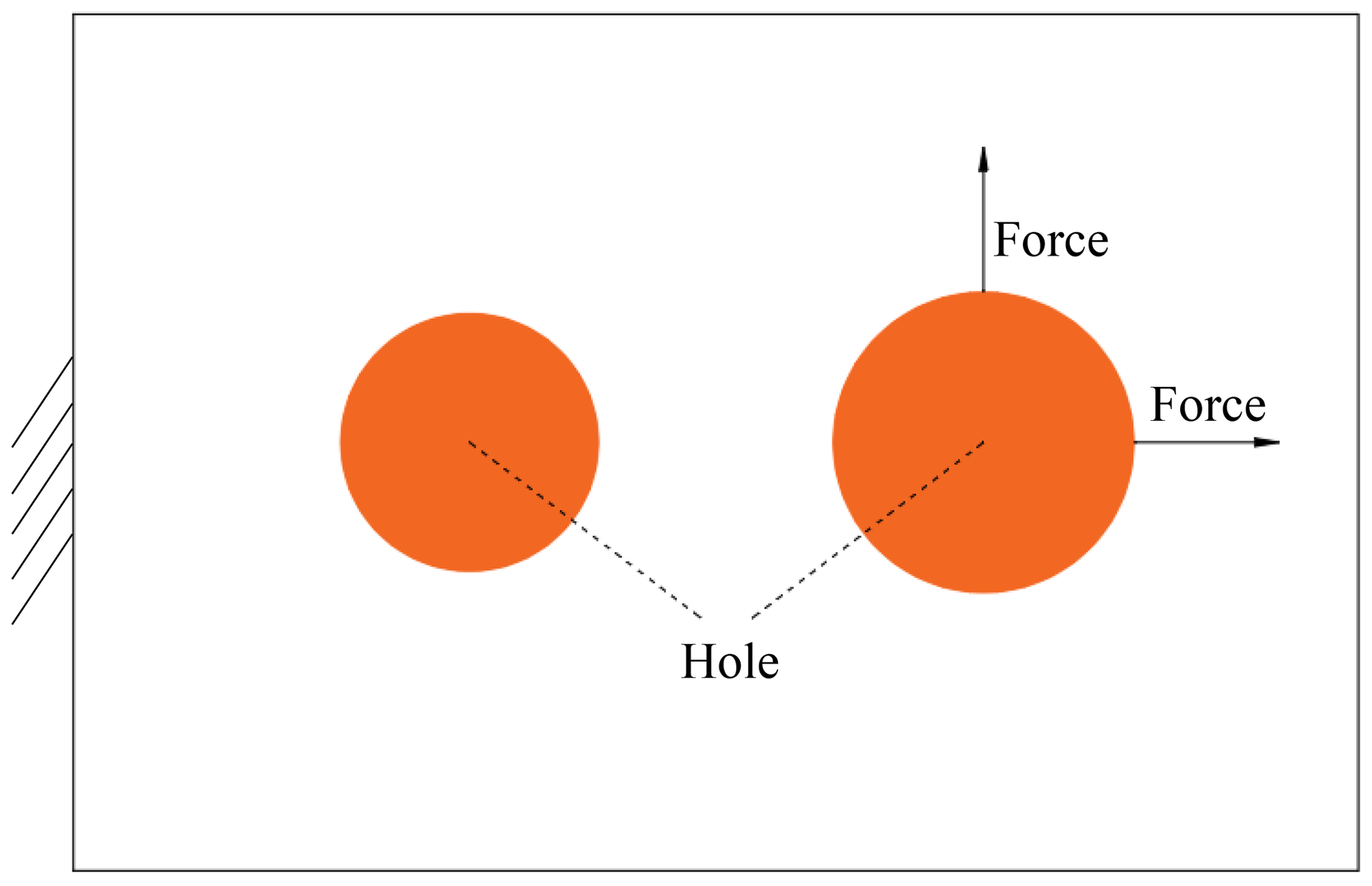
The design aim of the machine tool headstock is the same as the previous examples. The dimension of the considered headstock is $\mathrm{0.6}\mathrm{m}\times \mathrm{0.4}\mathrm{m}\times \mathrm{0.3}\mathrm{m}$. The finite element mesh of 120×80 elements is used. The two point loads are 1000 N. The motor in the left hole (diameter of 6 cm) and the spindle in the right hole (diameter of 7 cm) generate 1000 and 500 W thermal loads at their centers. The solid base material of the headstock is HT300. Young's modulus of the solid base material is 130 GPa, and Poisson’s ratio is 0.25. The thermal conductivity and the thermal expansion coefficient of the solid base material are 45 W m⁻¹ °C⁻¹ and $\mathrm{1.12}\times {\mathrm{10}}^{-\mathrm{5}}$ °C⁻¹. The reference temperature used is 0 °C. The radius of the sensitivity filter is 2.1 finite elements. All the temperature constraints are set in the centers of the holes.

5.3.1 Comparison of the different temperature constraints

In this section, the compliance of the machine tool headstock is minimized subject to a volume fraction constraint of 40 % and different temperature constraints of 80, 84, and 88 °C. The optimal topologies and the corresponding temperature distributions are shown in Fig. 14. Due to the greater thermal load generated by the motor in the left hole compared to the spindle in the right hole, more materials are distributed near the left hole. When the temperature constraint is 88 °C, the temperature at the center of the motor is higher than at the center of the spindle. Therefore, when the temperature constraint is enhanced, the materials that were originally distributed near the spindle are distributed near the motor. However, the compliance of the headstock has also been greatly improved at the same time.

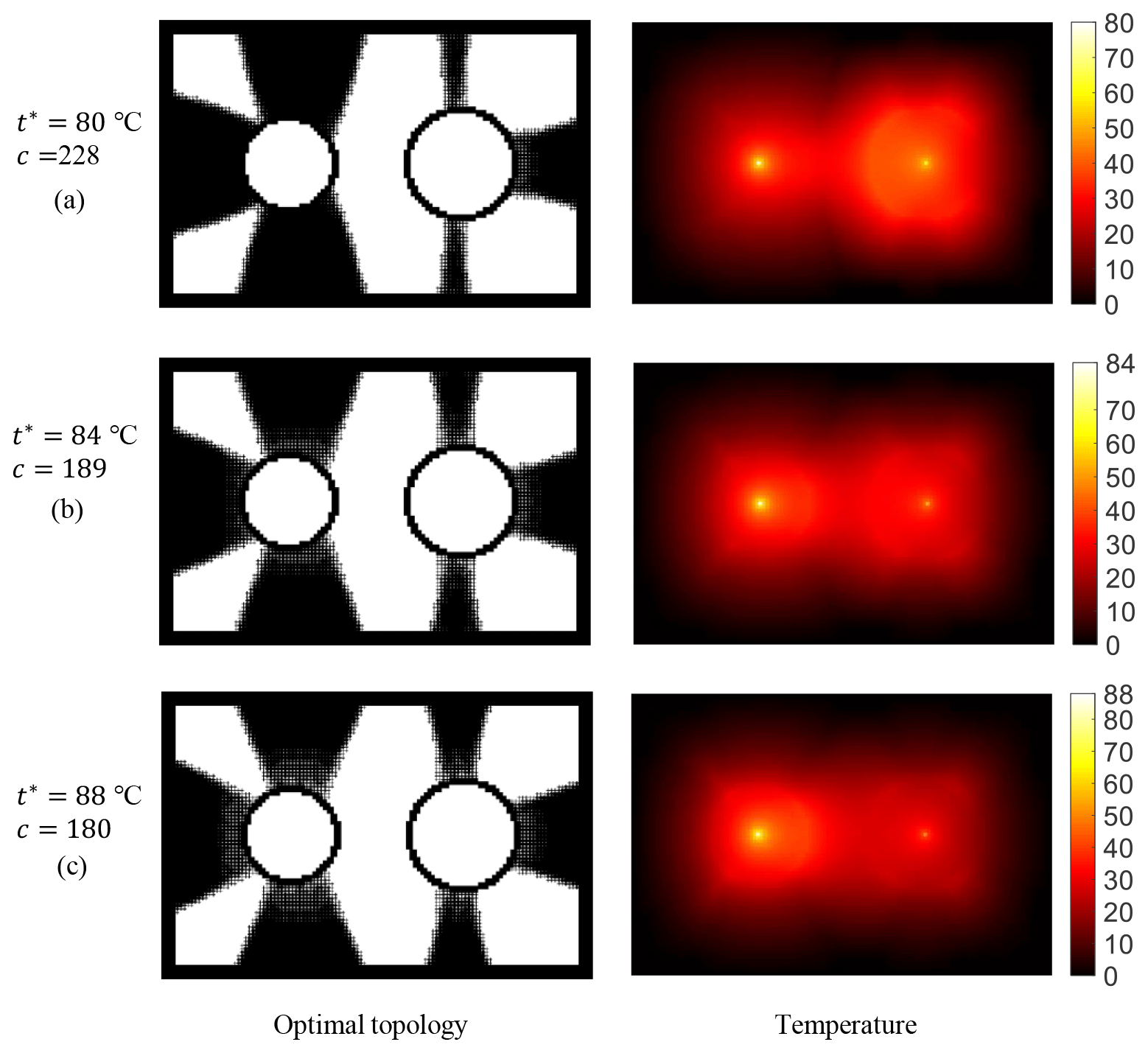
Figure 14 Optimal topologies and the corresponding temperature distributions subject to a volume fraction constraint of 40 % and different temperature constraints.

5.3.2 Comparison of different volume fraction constraints

In this section, the compliance of a machine tool headstock is minimized subject to the same temperature constraints of 80 °C and different volume fraction constraints of 50 %, 55 %, and 60 %, respectively. Optimal topologies and the corresponding temperature distributions obtained using the proposed approach are shown in Fig. 15. When the volume fraction constraint becomes weaker, the newly added material is distributed near the shortest heat dissipation path and the temperature and thermoelastic load of the headstock are thus reduced to the greatest extent, and finally the compliance is minimized under the corresponding design conditions.

Figure 15 Optimal topologies and the corresponding temperature distributions subject to a temperature constraint of 80 °C and different volume fraction constraints.

5.3.3 Comparison with solid structures

The headstock designed according to this paper is compared with the solid headstock in this part. Their objective functions, constraints, and discretizations are identical. The volume fraction and temperature constraint are 70 % and 80 °C, respectively. The optimal topology and the corresponding temperature distribution of the headstock obtained using solid-structure topology optimization and the proposed method are shown in Fig. 16. The compliance of the headstock obtained using the presented scheme is 9.0 % lower than that of the solid optimal topology, while their corresponding temperature distributions are similar. Since the thermal load generated in the left hole is much greater than that generated in the right hole, the temperature near the left hole is higher in both cases.

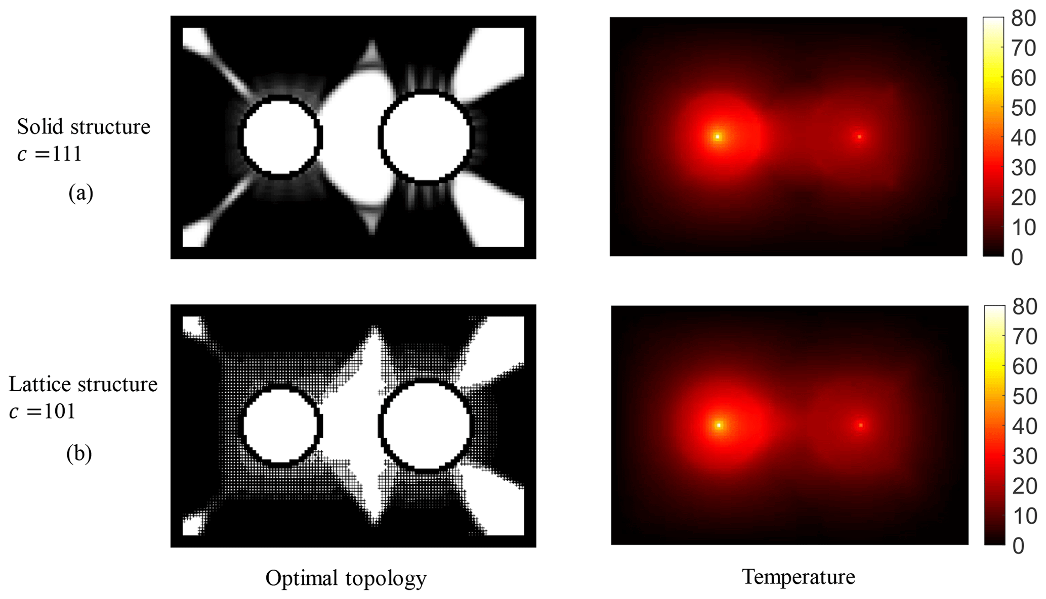
Figure 16 Optimal topologies and the corresponding temperature distributions subject to a volume fraction constraint of 70 % and a temperature constraint of 80 °C.

6 Conclusions

A thermomechanical coupled topology optimization for parameterized lattice structures is developed. The proposed approach integrates heat transfer and thermoelastic models and, unlike commonly used approximation methods, imposes precise temperature constraints on the structure. This framework enables the limitation of the maximum temperature of the structure and accounts for the influence of design variables on the temperature field distribution, bringing the optimized model more in line with the real world. By employing polynomial interpolation models, the method avoids the need for numerical homogenization during optimization iterations, thereby reducing computational costs. Numerical validation results for a battery pack, L-bracket, and machine tool headstock demonstrate that the proposed method accurately limits the temperature of structures and reduces their compliance by about 10 %–20 % compared to traditional solid-structure topology optimization. The examples show that, as temperature constraints become stricter, the material increases along the shortest path between the heat source and the constant temperature boundary, effectively reducing the maximum temperature while minimizing the structural compliance. If the proposed framework is extended from 2D to 3D, it can be applied in a wide range of fields in the real world, such as aircraft-bearing brackets, automotive battery brackets, and machine tool headstocks. These complex structures simultaneously bear mechanical and thermoelastic loads, and applying this framework will greatly enhance their performance. Additionally, considering the convection of these structures with external gases during optimization will yield even better results.

However, the computational cost of the proposed method is expensive because of the sensitivity calculation required for thermomechanical problems under design-dependent varying temperature field conditions. In this scenario, the sensitivity of compliance for the design variables includes the sensitivity of the temperature of each finite element to the design variables. It is a time-consuming process to determine the sensitivity of the temperature of each finite element to the design variables. Deep learning has been applied in various fields, such as hand gesture recognition for tele-operated robot and aircraft control (Qi et al., 2021; Zhao et al., 2022), and it may offer an effective solution to the aforementioned problem. In fact, deep learning has already had some applications in topology optimization (Yu et al., 2019; Deng et al., 2022), and it may help accelerate finite element analysis and sensitivity analysis. Additionally, incorporating lattices with different shapes into the topology optimization of structures may enhance their thermomechanical properties (Wang et al., 2021). When introducing different shapes of lattices during optimization, it may be a challenge to comprehensively compare the various types of properties of lattices with different shapes.