Research on anti-rollover control of three-axle rescue vehicle based on active suspension and differential braking

Due to its intricate operational environment, substantial mass and elevated center of mass, the three-axle emergency rescue vehicle is more prone to rollover. This study aims to enhance the operational stability and mitigate rollover risks by establishing a rollover dynamic model with 11 degrees of freedom. Using the coupling characteristics of vehicle dynamics and tire force, an anti-rollover control strategy of the three-axle vehicle based on the cooperative work of differential braking and active suspension is proposed. According to the vehicle motion characteristics, the active suspension controller is built using a fuzzy proportional–integral–derivative (PID) algorithm, and the differential braking controller is built using the improved adaptive model predictive control (MPC) algorithm. The step and fishhook tests of differential braking, active suspension control, and joint control are carried out. The simulation results show that the joint control strategy can effectively reduce the rollover tendency of the vehicle and further improve the anti-rollover ability of the vehicle compared with the single control system.

1 Introduction

For areas with complex terrain, frequent natural disasters and complex accident sites, modern emergency rescue vehicles should have higher performance requirements. At present, the common chassis technology and passive suspension system adopted have the problems of low off-road driving speed and poor handling performance. Therefore, there is a strong technical demand for the chassis technology and suspension system of emergency rescue vehicles.

The three-axle heavy rescue vehicle studied in this paper is characterized by large mass and high center of mass and is prone to rollover when encountering large corners and avoiding obstacles and other dangerous working conditions, so it is necessary to take the initiative to prevent rollover control of the vehicle (Huang et al., 2021). Many scholars have studied the problem of rollover control of the whole vehicle (e.g., Li and Tan, 2017). In a comprehensive manner, it seems that it is mainly through wheel braking/driving control (Chen and Peng, 2001a; Liang et al., 2020; Imine et al., 2015), active steering control (Son et al., 2017; Du et al., 2010; Shao et al., 2019; Yanhai, 2005; Azim et al., 2015) and active/semi-active suspension control (Yao et al., 2018; Riofrio et al., 2017) from different perspectives that improve the stability of the vehicle and enhance the active safety of the vehicle. In fact, each method has certain limitations.

In collaboration with heavy machinery companies, our team has designed and built a three-axle rescue vehicle with a new special chassis design and active suspension system. Great results have been achieved in key technologies, such as system dynamics models, integrated control algorithms and road environmental awareness. Several tests have been conducted on the maneuverability, smoothness and safety of the three-axle rescue vehicle (Chen et al., 2021; Liu et al., 2022; Ni et al., 2020; Wang et al., 2018). Figure 1 shows the team's three-axle rescue vehicle and the unpaved road surface.

Figure 1 (a) The three-axle rescue vehicle and (b) the unpaved road surface.

This paper proposes the combination of differential braking and active suspension control system to improve the anti-rollover capability of the three-axle rescue vehicle as the goal, and based on an 11-degree-of-freedom rollover dynamics model, the effectiveness and superiority of the integrated control methods and strategies are verified by simulating and comparing the braking and active suspension system controls separately and the joint control of the two.

1.1 11-degree-of-freedom vehicle rollover dynamics model

The vehicle rollover dynamics model mainly considers the lateral and vertical motions of the vehicle, the rotational motions around each axis in the vehicle coordinate system (transverse pendulum motion, pitch motion, and lateral tilt motion), and the vertical motion of the six wheels, with a total of 11 degrees of freedom, and it is shown in Fig. 2. In this paper, the controllable active suspension and independent braking system are used as actuators and the longitudinal speed of the three-axis vehicle during braking is used as a known input.

Figure 2 Vehicle rollover dynamics model with 11 degrees of freedom.

According to the 11-degree-of-freedom rollover dynamics model, there are several types of motion to consider, the first one being lateral motion:

$$\begin{array}{}\text{(1)}& \begin{array}{rl}mv& \left(\dot{\mathit{\beta }}+\mathit{\omega }\right)-m_{\mathrm{s}}{h}_{\mathrm{s}}\ddot{\mathit{\phi }}=\left(F_{y\mathrm{11}}+F_{y\mathrm{12}}\right)\cos \mathit{\delta }\\ & +F_{y\mathrm{21}}+F_{y\mathrm{22}}+F_{y\mathrm{31}}+F_{y\mathrm{32}}.\end{array}\end{array}$$

The second kind of motion is the yawing motion:

$$\begin{array}{}\text{(2)}& \begin{array}{rl}{I}_{zz}\dot{\mathit{\omega }}& =l_{\mathrm{1}}\left(F_{y\mathrm{11}}+F_{y\mathrm{12}}\right)\cos \mathit{\delta }-l_{\mathrm{2}}\left(F_{y\mathrm{21}}+F_{y\mathrm{22}}\right)\\ & -l_{\mathrm{3}}\left(F_{y\mathrm{31}}+F_{y\mathrm{32}}\right)+w_z.\end{array}\end{array}$$

The third type is the rolling motion:

$$\begin{array}{}\text{(3)}& \begin{array}{rl}{I}_{xx}& \dot{\mathit{\phi }}-m_{\mathrm{s}}{h}_{\mathrm{s}}v\left(\mathit{\omega }+\dot{\mathit{\beta }}\right)={\displaystyle \frac{b_{\mathrm{1}}}{\mathrm{2}}}\left(F_{\mathrm{11}}-F_{\mathrm{12}}\right)\\ & +{\displaystyle \frac{b_{\mathrm{2}}}{\mathrm{2}}}\left(F_{\mathrm{21}}-F_{\mathrm{22}}\right)+{\displaystyle \frac{b_{\mathrm{3}}}{\mathrm{2}}}\left(F_{\mathrm{31}}-F_{\mathrm{32}}\right)+m_{\mathrm{s}}g{h}_{\mathrm{s}}\mathit{\phi }.\end{array}\end{array}$$

Next comes the pitching motion:

$$\begin{array}{}\text{(4)}& \begin{array}{rl}{I}_{yy}& \ddot{\mathit{\theta }}-m_{\mathrm{s}}g{h}_{\mathrm{s}}\mathit{\theta }-l_{\mathrm{1}}\left(F_{\mathrm{11}}+F_{\mathrm{12}}\right)+l_{\mathrm{2}}\left(F_{\mathrm{21}}+F_{\mathrm{22}}\right)\\ & +l_{\mathrm{3}}\left(F_{\mathrm{31}}+F_{\mathrm{32}}\right)=\mathrm{0}.\end{array}\end{array}$$

There is also the vertical motion of sprung mass:

$$\begin{array}{}\text{(5)}& m_{\mathrm{s}}{\ddot{z}}_m=-F_{\mathrm{11}}-F_{\mathrm{12}}-F_{\mathrm{21}}-F_{\mathrm{22}}-F_{\mathrm{31}}-F_{\mathrm{32}}.\end{array}$$

Another kind is the vertical motion of unsprung mass:

$$\begin{array}{}\text{(6)}& m_u{\ddot{z}}_{uij}-F_{ij}+F_{tij}=\mathrm{0}.\end{array}$$

One more type is suspension force:

$$\begin{array}{}\text{(7)}& F_{ij}=k_s\left(z_{uij}-z_{sij}\right)+c_s\left({\dot{z}}_{uij}-{\dot{z}}_{sij}\right)+f_{ij}.\end{array}$$

The penultimate kind is tire force:

$$\begin{array}{}\text{(8)}& F_{tij}=k_{\mathrm{t}}(z_{rij}-z_{uij}).\end{array}$$

The final type is suspension displacement:

$$\begin{array}{}\text{(9)}& \begin{array}{rl}& z_{s\mathrm{11}}=z_m-l_{\mathrm{1}}\mathit{\theta }+{\displaystyle \frac{b_{\mathrm{1}}}{\mathrm{2}}}\mathit{\phi },z_{s\mathrm{12}}=z_m-l_{\mathrm{1}}\mathit{\theta }+{\displaystyle \frac{b_{\mathrm{1}}}{\mathrm{2}}}\mathit{\phi },\\ & z_{s\mathrm{21}}=z_m+l_{\mathrm{2}}\mathit{\theta }+{\displaystyle \frac{b_{\mathrm{2}}}{\mathrm{2}}}\mathit{\phi },z_{s\mathrm{22}}=z_m+l_{\mathrm{2}}\mathit{\theta }-{\displaystyle \frac{b_{\mathrm{2}}}{\mathrm{2}}}\mathit{\phi },\\ & z_{s\mathrm{31}}=z_m+l_{\mathrm{3}}\mathit{\theta }+{\displaystyle \frac{b_{\mathrm{3}}}{\mathrm{2}}}\mathit{\phi },z_{s\mathrm{32}}=z_m+l_{\mathrm{3}}\mathit{\theta }-{\displaystyle \frac{b_{\mathrm{3}}}{\mathrm{2}}}\mathit{\phi }.\end{array}\end{array}$$

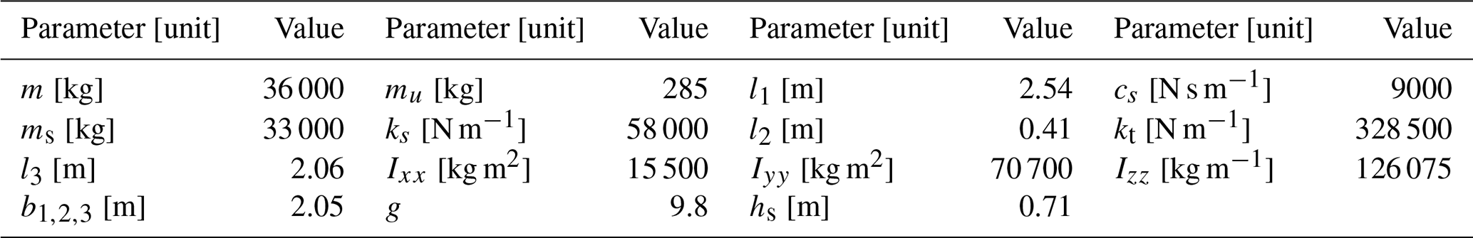
The specific parameters of the vehicle are shown in Table 1. The value is obtained by the test conducted by our team.

Table 1 Parameters of the three-axle vehicle rollover dynamics model.

1.2 Tire model of the differential braking for anti-rollover control of the three-axle vehicle

In the process of using differential braking for anti-rollover control of the three-axle vehicle, the linear tire force model cannot meet the requirements. In order to better represent the nonlinear mechanical characteristics of tires, this paper uses the “magic formula” tire model (Yu and Lin, 2016) and the concept of the tire attachment ellipse to demonstrate (Arat et al., 2014).

The magic formula is proposed and developed by professor H. B. Pacejka and their colleagues. It is a mathematical model of the longitudinal force, lateral force and return moment of the tire established by a combination of trigonometric formulas (Dukkipati et al., 2008). Since only a set of formulas can express the complete set of force characteristics of the tire under pure working conditions, we need to use the so-called magic formula. The general formulation of the magic formula is

$$\begin{array}{}\text{(10)}& \begin{array}{rl}F& =D\cdot \sin \left(C\cdot \arctan \left(B\cdot x\right.\right.\\ & \left.\left.-E\cdot \left(B\cdot x-\arctan (B\cdot x)\right)\right)\right)+S_v.\end{array}\end{array}$$

The tire data selected in this paper come from TruckSim's (or CarSim's) “3000 kg rating, 510 mm radius” tire type, and the Simulink (MathWorks) tire model is fitted to the known data according to the magic formula to compare the results, as shown in Fig. 3.

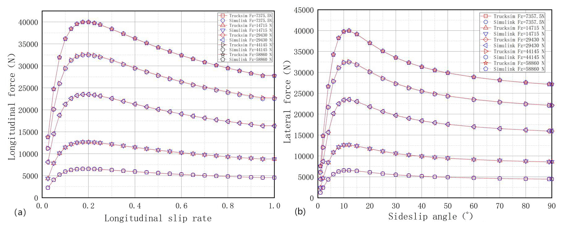
Figure 3 Tire-fitting curves: (a) tire longitudinal force curve and (b) tire lateral force curve.

1.3 Tire force analysis

There are three main forces acting on the tires: longitudinal force, vertical force and lateral force. In the case of a vehicle moving at a constant speed on a curved route, the main consideration when analyzing the tires is the vertical and lateral forces affecting the vehicle. When the vehicle is accelerating or braking during the curve movement, the longitudinal force, vertical force and lateral force must be considered at the same time. The three forces affect each other and are mutually constrained. The relationship between the three forces can be described by the concept of the tire attachment ellipse (Chen and Peng, 2001b), as shown in Fig. 4.

Figure 4 Tire attachment ellipse.

The relationship between the longitudinal force and the lateral deflection force of the tire can be obtained from the characteristics of the tire force attachment ellipse as follows:

$$\begin{array}{}\text{(11)}& {\left({\displaystyle \frac{F_{xij}}{F_{xij\max }}}\right)}^{\mathrm{2}}+{\left({\displaystyle \frac{F_{yij}}{F_{yij\max }}}\right)}^{\mathrm{2}}=\mathrm{1}(i=\mathrm{1}--\mathrm{3},j=\mathrm{1}--\mathrm{2}),\end{array}$$

where F_xijmax and F_yijmax are the maximum longitudinal force and lateral deflection force of each tire, respectively. The maximum longitudinal force of the tire is determined by the tire adhesion, which is expressed by

$$\begin{array}{}\text{(12)}& F_{xij\max }=\mathit{\mu }{F}_{zij}(i=\mathrm{1}--\mathrm{3},j=\mathrm{1}--\mathrm{2}),\end{array}$$

where μ is the coefficient of adhesion of the tire to the ground. The maximum lateral deflection force of a tire with large lateral acceleration and large lateral deflection angle, F_yijmax, can be considered to be the lateral deflection force of that tire when there is no longitudinal force at a certain lateral deflection angle. In this case, the lateral force of the tire can be considered to have reached the adhesion limit.

The lateral deflection force of each tire, F_yijmax, is calculated according to the magic formula in the previous section.

2 Vehicle rollover dynamic stability evaluation index

When the vehicle is driving in a high-speed turn, the vertical load of the tires will be displaced laterally, the load on the inner tires will be reduced and the load on the outer tires will be increased; when the inner load is reduced to zero and the tires are not in contact with the ground, once there is lateral interference, the vehicle will roll over. Therefore, the tire load transfer ratio (LTR) can be used as the dynamic stability evaluation index of vehicle rollover (Larish et al., 2013). LTR is simple and effective as an indicator for evaluating vehicle rollover stability.

$$\begin{array}{}\text{(13)}& \mathrm{LTR}={\displaystyle \frac{\left|F_{z\mathrm{11}}+F_{z\mathrm{21}}+F_{z\mathrm{31}}-F_{z\mathrm{12}}-F_{z\mathrm{22}}-F_{z\mathrm{32}}\right|}{F_{z\mathrm{11}}+F_{z\mathrm{21}}+F_{z\mathrm{31}}+F_{z\mathrm{12}}+F_{z\mathrm{22}}+F_{z\mathrm{32}}}},\end{array}$$

where F_z11, F_z21 and F_z31 are the vertical load of the left wheels and F_z12, F_z22 and F_z32 are the vertical load of the right wheels, the value of LTR is from 0 to 1, the smaller the value of LTR means the smoother the vehicle driving.

The vertical load on the wheels F_zij ($i=\mathrm{1},\mathrm{\dots },\mathrm{3}$; $j=\mathrm{1},\mathrm{\dots },\mathrm{2}$) can be derived from the static vertical load on the wheels plus the value of the suspension force variation. Combined with the vehicle side defense dynamics model, the expression of the new LTR can be obtained as follows:

$$\begin{array}{}\text{(14)}& \left\{\begin{array}{l}\mathrm{LTR}=\frac{\mathrm{2}\left(I_x\ddot{\mathit{\phi }}-m_{\mathrm{s}}{a}_y{h}_{\mathrm{s}}-m_{\mathrm{s}}g{h}_{\mathrm{s}}\mathit{\phi }\right)}{Bmg},\\ B=\frac{b_{\mathrm{1}}+b_{\mathrm{2}}+b_{\mathrm{3}}}{\mathrm{3}}.\end{array}\right.\end{array}$$

3 Anti-rollover control strategy research

3.1 Joint control strategy

According to the tire dynamics coupling relationship, the longitudinal force and lateral force of the wheel are both functions of the vertical load of the wheel, and the magnitude of the additional yaw moment generated by differential braking is also related to the vertical load of the braking wheel, which can be adjusted by controlling the actuation force of the suspension system. In order to suppress the occurrence of vehicle rollover more effectively, this paper designs a three-axis vehicle active anti-rollover control system based on active suspension and differential braking joint control, and the overall structure of the control system is shown in Fig. 5 below.

Figure 5 Joint control.

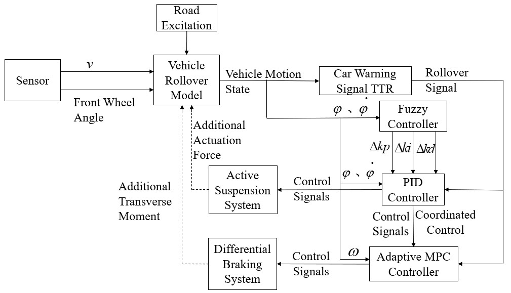
The joint control process is as follows: (1) The vehicle longitudinal speed, front-wheel angle signals, road excitation signals, and the controller output signals (additional actuation force signals and additional torque signals) from the previous round of control process are used as inputs to the vehicle rollover dynamics equations, and the vehicle motion parameter signals (rollover angle, rollover angular velocity, cross-swing angular velocity, lateral angular velocity) are solved. (2) Obtain the LTR value based on the settled vehicle motion parameters and the calculation equations. (3) The LTR value and vehicle motion parameters are used as input to the joint controller, which processes them to obtain the control signals for the active suspension and differential braking. (4) The actuator receives the control signal and executes the corresponding action to control the differential braking and active suspension of the vehicle. The anti-rollover function is realized and provides the output signal of the controller for the next round of control to achieve closed-loop control.

3.2 Active suspension control strategy based on fuzzy PID

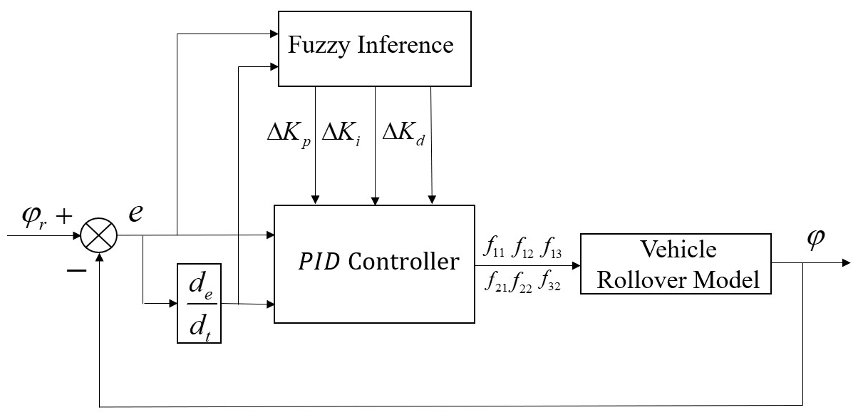
The vehicle system is a nonlinear and multicoupled system. It is difficult to establish a completely accurate mathematical model. The fuzzy proportional–integral–derivative (PID) control method has good robustness and does not require a high-order mathematical model (Verma et al., 2018). In this paper, the difference between the roll angle and the ideal roll angle as well as the difference between the roll angle rate and the ideal roll rate are taken to be the input of the fuzzy PID controller, and the power is taken to be the output of the controller.

The fuzzy PID controller consists of two parts: the fuzzy controller part and the PID controller part. The fuzzy controller adjusts the values of the parameters ΔK_p, ΔK_i and ΔK_d according to the difference between the roll angle and the ideal roll angle and the rate of change in the difference. The PID controller parameters, K_p, K_i and K_d, are adjusted in real time according to the results obtained from the fuzzy controller. The PID controller output is the actuation force of the left- and right-side suspensions of the vehicle. The control structure of the fuzzy PID is shown in Fig. 6.

Figure 6 Fuzzy PID control structure diagram.

The fuzzy control strategy uses fuzzy logic and approximate reasoning to output the required control quantities for effective control of the target. The input variables e and ec and output variables correspond to fuzzy quantities of E, EC and U, respectively.

The fuzzy subset of E is $\left\{\mathrm{NB},\mathrm{NM},\mathrm{NS},\mathrm{ZO},\mathrm{PS},\mathrm{PM},\mathrm{PB}\right\}$, where the members of the subset are defined as negative large (NB), negative medium (NM), negative small (NS), almost zero (ZO), positive small (PS), positive medium (PM) and positive large (PB). The fuzzy subset of EC is $\left\{\mathrm{NB},\mathrm{NM},\mathrm{NS},\mathrm{ZO},\mathrm{PS},\mathrm{PM},\mathrm{PB}\right\}$, and the fuzzy subset of U is $\left\{\mathrm{NB},\mathrm{NM},\mathrm{NS},\mathrm{ZO},\mathrm{PS},\mathrm{PM},\mathrm{PB}\right\}$. The error, E, and the rate of change in the error, EC, are set to $\left[-\mathrm{3},\mathrm{3}\right]$, and the output signals, ΔK_p, ΔK_i and ΔK_d are set to $\left[-\mathrm{3},\mathrm{3}\right]$, $\left[-\mathrm{10},\mathrm{0}\right]$ and [0,1], respectively. The fuzzy rules are listed in Table 2.

Table 2 Fuzzy rules.

3.3 Differential braking control strategy based on adaptive model prediction

The differential-braking-based stability control method for three-axle heavy vehicles is developed on the basis of a system which collects the error feedback between the actual driving state of the vehicle and the ideal state, decides the additional yaw moment required for the stability of a three-axle heavy vehicle, and obtains the required additional yaw moment by applying braking force to different wheels to achieve the anti-rollover control of a three-axle heavy vehicle. The adaptive control structure diagram is shown in Fig. 7.

Figure 7 Adaptive model predictive control (MPC) control structure diagram.

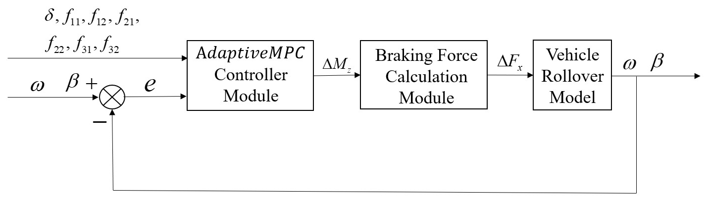
The differential brake control system based on adaptive model prediction consists of two main parts, one of which is the upper adaptive controller part. The upper adaptive model predictive control (MPC) controller takes the difference between the desired yaw angle rate and the vehicle body sideslip angle obtained from the ideal model and the actual value output from Simulink's three-axis rollover dynamics model as the input to the adaptive control algorithm and the additional yaw moment required for vehicle stability as the output. The quadratic programming algorithm is used to solve for the optimized objective function and constraints in the model predictive control algorithm. The second is the lower braking force calculation module, which receives the additional yaw moment signal from the upper adaptive MPC controller and calculates the braking force of the target wheel based on the braking force calculation module.

3.4 Adaptive MPC controller design

The design of the adaptive MPC-based additional transverse moment controller consists of the following parts: the determination of the vehicle model and derivation of the prediction equations, determination of the objective function and control constraints, and constraint optimization solution (Mata et al., 2017).

Determination of the vehicle model and derivation of the prediction equation. The prediction model of the MPC control method based on the state equation is a linear state space equation, and the previous three-axis rollover dynamics model cannot be used directly in the prediction model because the tire lateral force is nonlinear; therefore, the adaptive MPC controller is proposed in this paper. The structure of the adaptive MPC controller designed in this paper is shown in Fig. 8, which is divided into the MPC controller, a state matrix update module and a parameter estimation module.

Figure 8 Adaptive MPC controller structure diagram.

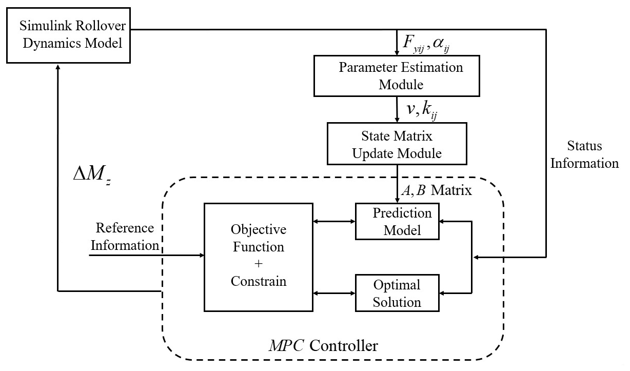
The state matrix update module is an important part necessary to reflect the adaptive capability because the Simulink rollover dynamics model established in this paper is time-varying and nonlinear, its parameters (vehicle longitudinal velocity, v, and lateral deflection stiffness of six wheels) change in real time, and the prediction model needs to be updated in real time for the accuracy of controller control. In the state update module, we assume that the state matrix is constant within one calculation cycle, and outside one calculation cycle, the state matrix is updated by the state matrix update module. The parameter estimation module is used to estimate the real-time longitudinal speed of the vehicle, v, and the lateral deflection stiffness of the six wheels.

$$\begin{array}{}\text{(15)}& F_{yij}=k_{ij}{\mathit{\alpha }}_{ij},\end{array}$$

where F_yij ($i=\mathrm{1},\mathrm{\dots },\mathrm{3}$; $j=\mathrm{1},\mathrm{\dots },\mathrm{2}$) is the lateral deflection force of each wheel, k_ij is the lateral deflection stiffness of each wheel and α_ij is the lateral deflection angle of each wheel.

The status variables are as follows:

$$\begin{array}{rl}x=& \left[z_m{\dot{z}}_m{z}_{u\mathrm{11}}{\dot{z}}_{u\mathrm{11}}{z}_{u\mathrm{12}}{\dot{z}}_{u\mathrm{12}}{z}_{u\mathrm{21}}{\dot{z}}_{u\mathrm{21}}{z}_{u\mathrm{22}}{\dot{z}}_{u\mathrm{22}}{z}_{u\mathrm{31}}{\dot{z}}_{u\mathrm{31}}\right.\\ & {\left.z_{u\mathrm{32}}{\dot{z}}_{u\mathrm{32}}\mathit{\theta }\dot{\mathit{\theta }}\mathit{\phi }\dot{\mathit{\phi }\mathit{\beta }\mathit{\omega }}\right]}^T.\end{array}$$

The input volume is u=[δ Δω_z f₁₁f₁₂ f₂₁f₂₂ f₃₁f₃₂ z₁₁z₁₂ z₂₁z₂₂ z₃₁z₃₂], and the output, the active suspension's force, f₁₁, f₁₂, f₂₁, f₂₂, f₃₁ and f₃₂, is taken to be the input to the adaptive MPC, which is the method for achieving joint control in this paper.

The status matrix can be formulated as A=[A₁A₂], B=[B₁B₂] and $C=\left[Z_{\mathrm{4}\times \mathrm{20}}{Z}_{\mathrm{2}\times \mathrm{18}}{I}_{\mathrm{2}\times \mathrm{2}}\right]$; matrices A₁, A₂, B₁ and B₂ are shown at the end of this paper; Z_6×14 is a zero matrix with 6 rows and 14 columns; and I_6×6 is a unit matrix with six rows and six columns.

Forward Eulerian discretization of the system is performed, and the state prediction equation based on time is developed.

$$\begin{array}{}\text{(16)}& \left\{\begin{array}{l}x\left(\left.k+\mathrm{1}\right|k\right)=A\left(k\mathrm{|}k\right)x\left(k\mathrm{|}k\right)+B\left(k\mathrm{|}k\right)u\left(k\mathrm{|}k\right)\\ y=C\left(k\mathrm{|}k\right)x\left(k\mathrm{|}k\right)\end{array}\right.\end{array}$$

$$\left\{\begin{array}{l}A\left(k\mathrm{|}k\right)=I+TA\\ B\left(k\mathrm{|}k\right)=TB\\ C\left(k\mathrm{|}k\right)=C\end{array}\right.$$

In order to reduce the computational complexity of the MPC controller to improve computational efficiency, the following assumptions are made in this paper:

$$\left\{\begin{array}{l}A\left(k\mathrm{|}k\right)=A\left(t\mathrm{|}k\right),t=k,k+\mathrm{1},\mathrm{\cdots },k+p-\mathrm{1},\\ B\left(k\mathrm{|}k\right)=B\left(t\mathrm{|}k\right),t=k,k+\mathrm{1},\mathrm{\cdots },k+p-\mathrm{1},\end{array}\right.$$

where p is the set prediction step. We predict p moments after moment k and obtain the new prediction equation:

$$\begin{array}{}\text{(17)}& \left\{\begin{array}{l}{X}_p\left(k+p\mathrm{|}k\right)=\stackrel{\mathrm{‾}}{A}x\left(k\mathrm{|}k\right)+\stackrel{\mathrm{‾}}{B}{U}_c,\\ Y_p\left(k+p\mathrm{|}p\right)=\mathrm{\Psi }x\left(k\mathrm{|}k\right)+\mathrm{\Theta }{U}_c.\end{array}\right.\end{array}$$

Among them, the following applies:

$$\begin{array}{rl}& X_p\left(k+p\mathrm{|}p\right)=\left[\begin{array}{l}x\left(k+\mathrm{1}\mathrm{|}k\right)\\ x\left(k+\mathrm{2}\mathrm{|}k\right)\\ \mathrm{⋮}\\ x(k+p\mathrm{|}k)\end{array}\right],\\ & Y_p\left(k+p\mathrm{|}k\right)=\left[\begin{array}{l}y\left(k+\mathrm{1}\mathrm{|}k\right)\\ y\left(k+\mathrm{2}\mathrm{|}k\right)\\ \mathrm{⋮}\\ y(k+p\mathrm{|}k)\end{array}\right],\\ & U_c=\left[\begin{array}{l}u\left(k\right)\\ u\left(k+\mathrm{1}\right)\\ \mathrm{⋮}\\ u(k+c-\mathrm{1})\end{array}\right].\end{array}$$

Here, p is the prediction time domain, the value of which is 10; c is the control time domain, the value of which is 3; x(k+1|k), $x\left(\left.k+\mathrm{2}\right|k\right),\mathrm{\dots },x\left(\left.k+p\right|k\right)$ are the predicted state variable values for each step in the prediction time domain at moment k; y(k+1|k), $y\left(\left.k+\mathrm{2}\right|k\right),\mathrm{\dots },y\left(\left.k+p\right|k\right)$ are the predicted output values for each step in the prediction time domain at moment k; and u(k), $u(k+\mathrm{1}),\mathrm{\dots },u(k+c-\mathrm{1})$ are the expected input values for each step in the control time domain at moment k. The prediction matrices, $\stackrel{\mathrm{‾}}{A}$, Ψ, $\stackrel{\mathrm{‾}}{B}$ and Θ, are specified as follows, respectively:

$$\stackrel{\mathrm{‾}}{A}=\left[\begin{array}{l}A\left(k\mathrm{|}k\right)\\ A^{\mathrm{2}}\left(k\mathrm{|}k\right)\\ \mathrm{⋮}\\ A^p\left(k\mathrm{|}k\right)\end{array}\right],\mathrm{\Psi }=\left[\begin{array}{l}C\left(k\mathrm{|}k\right)A\left(k\mathrm{|}k\right)\\ C\left(k\mathrm{|}k\right)A^{\mathrm{2}}\left(k\mathrm{|}k\right)\\ \mathrm{⋮}\\ C\left(k\mathrm{|}k\right)A^p\left(k\mathrm{|}k\right)\end{array}\right],$$

$\stackrel{\mathrm{‾}}{B}=\left[\begin{array}{c}\begin{array}{cccc}B\left(k\mathrm{|}k\right)& \mathrm{0}& \mathrm{\cdots }& \mathrm{0}\\ A\left(k\mathrm{|}k\right)B\left(k\mathrm{|}k\right)& B\left(k\mathrm{|}k\right)& \mathrm{\cdots }& \mathrm{0}\\ \mathrm{⋮}& \mathrm{⋮}& \mathrm{\ddots }& \mathrm{⋮}\\ A^{c-\mathrm{1}}\left(k\mathrm{|}k\right)B\left(k\mathrm{|}k\right)& A^{c-\mathrm{2}}\left(k\mathrm{|}k\right)B\left(k\mathrm{|}k\right)& \mathrm{\cdots }& B\left(k\mathrm{|}k\right)\\ \mathrm{⋮}& \mathrm{⋮}& \mathrm{⋮}& \mathrm{⋮}\\ A^{p-\mathrm{1}}\left(k\mathrm{|}k\right)B\left(k\mathrm{|}k\right)& A^{p-\mathrm{2}}\left(k\mathrm{|}k\right)B\left(k\mathrm{|}k\right)& \mathrm{\cdots }& A^{p-c}\left(k\mathrm{|}k\right)B\left(k\mathrm{|}k\right)\end{array}\end{array}\right],$
$\mathrm{\Theta }=\left[\begin{array}{cccc}C\left(k\mathrm{|}k\right)B\left(k\mathrm{|}k\right)& \mathrm{0}& \mathrm{\cdots }& \mathrm{0}\\ C\left(k\mathrm{|}k\right)A\left(k\mathrm{|}k\right)B\left(k\mathrm{|}k\right)& C\left(k\mathrm{|}k\right)B\left(k\mathrm{|}k\right)& \mathrm{\cdots }& \mathrm{0}\\ \mathrm{⋮}& \mathrm{⋮}& \mathrm{\ddots }& \mathrm{⋮}\\ C\left(k\mathrm{|}k\right)A^{c-\mathrm{1}}\left(k\mathrm{|}k\right)B\left(k\mathrm{|}k\right)& C\left(k\mathrm{|}k\right)A^{c-\mathrm{2}}\left(k\mathrm{|}k\right)B\left(k\mathrm{|}k\right)& \mathrm{⋮}& \mathrm{⋮}\\ \mathrm{⋮}& \mathrm{⋮}& \mathrm{⋮}& \mathrm{⋮}\\ C\left(k\mathrm{|}k\right)A^{p-\mathrm{1}}\left(k\mathrm{|}k\right)B\left(k\mathrm{|}k\right)& C\left(k\mathrm{|}k\right)A^{p-\mathrm{2}}\left(k\mathrm{|}k\right)B\left(k\mathrm{|}k\right)& \mathrm{\cdots }& C\left(k\mathrm{|}k\right)A^{p-c}\left(k\mathrm{|}k\right)B\left(k\mathrm{|}k\right)\end{array}\right]$

Design of the final optimization objective function. By optimally solving the objective function, a series of optimal control inputs can be obtained which will act the first component on the system. The objective function designed in this paper is as follows:

$$\begin{array}{}\text{(18)}& \begin{array}{rl}J\left(U_c\right)& =\sum _{i=\mathrm{1}}^p{∥y\left(k+i\mathrm{|}k\right)-y_{\mathrm{ref}}(k+i\mathrm{|}k)∥}_Q^{\mathrm{2}}\\ & +\sum _{j=\mathrm{0}}^{c-\mathrm{1}}{∥u(k+j)∥}_R^{\mathrm{2}}.\end{array}\end{array}$$

In the above equation, $y_{\mathrm{ref}}\left(k+i\mathrm{|}k\right),i=\mathrm{1},\mathrm{2},\mathrm{\dots },p$, is the information on the reference ideal transverse pendulum angular velocity and the lateral deflection of the center of mass. Q and R are the penalty matrix of the process state and control input quantity. In this paper, the ideal reference information module is derived.

In order to ensure the safety of driving the three-axis vehicle, the control input (the additional yaw moment) to be achieved is constrained, and the expression of the constraint is as follows:

$$\begin{array}{}\text{(19)}& u_{\min }\le u\left(k+j\mathrm{|}k\right)\le u_{\max },j=\mathrm{0},\mathrm{1},\mathrm{\dots },c-\mathrm{1}.\end{array}$$

The maximum and minimum values of the additional transverse moment here can be derived from Sect. 1.3 in this paper.

Figure 9 Working front-wheel rotation angle.

Figure 10 LTR.

Figure 11 Roll angle.

Figure 12 Lateral acceleration.

4 Simulation results

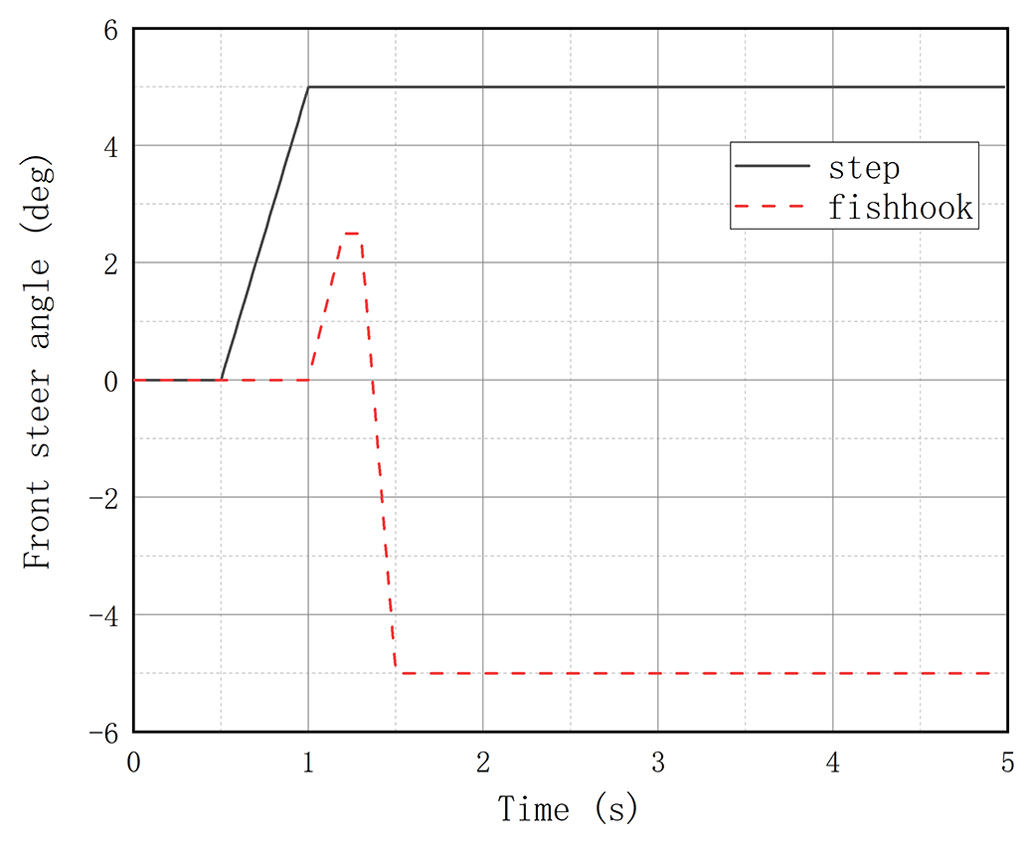
In the previous section, a coordinated control strategy for the lateral dynamics of the three-axis rescue vehicle was proposed. In this section, two suitable simulation test conditions were set up in the MATLAB/Simulink environment to verify the effectiveness of the proposed control strategy. MATLAB, short for Matrix Laboratory, is a commercial mathematical software by MathWorks, a US-based company that provides an advanced technical computing language and interactive environment for algorithm development, data visualization, data analysis and numerical computation, consisting of two main components: MATLAB and Simulink. One of the most popular international software tools for scientific and engineering computing, Simulink, supports system-level design, simulation, automated code generation, and continuous testing and verification of embedded systems. Simulink is integrated with MATLAB and works with MATLAB in an integrated way, allowing for MATLAB algorithms to be used and exported to MATLAB for further analysis. The simulation software version for this paper is MATLAB 2021b. The hardware configuration is a Windows-based computer with an Intel Core i7-10750H processor and 12GB of running memory. The step and fishhook conditions are selected for the simulation, and the “no control”, “single control” and “joint control” strategies are simulated for each condition, where no control means the vehicle controller is turned off for the simulation test, single control means the vehicle is simulated with the active suspension controller and the differential brake controller turned on, and joint control means the vehicle is simulated with both the active suspension controller and the differential brake controller turned on. The front-wheel angles for both conditions are shown in Fig. 9.

4.1 Step-steering simulation

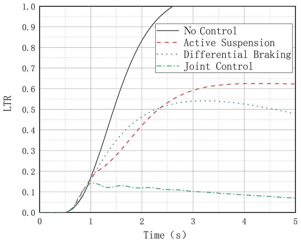
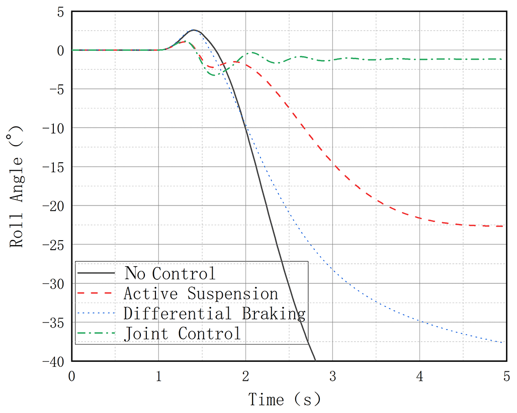
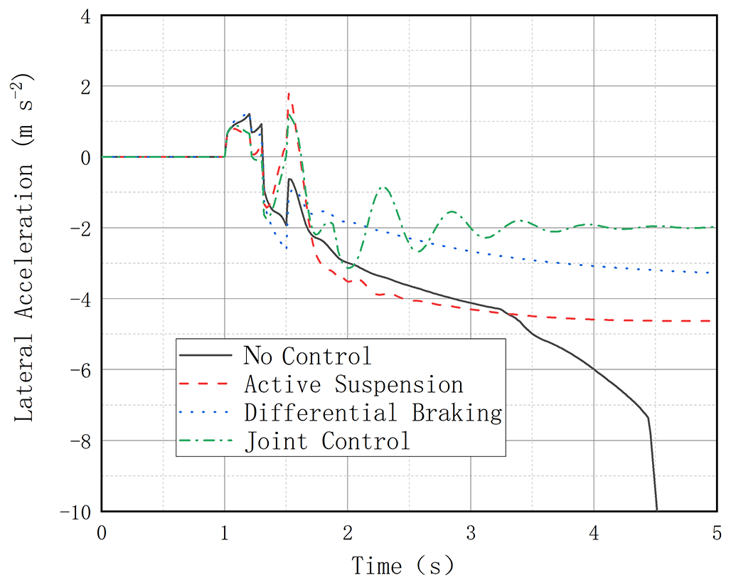
The step-steering test was carried out under the road condition with an adhesion coefficient of 0.8. The maximum speed of the designed three-axle rescue vehicle is 100 km h⁻¹, and the simulation speed is set to 60 km h⁻¹; the front-wheel turning angle is the step-turning angle, the start time is 0.5 s, the duration is 0.5 s, and the maximum front-wheel turning angle input is 6°. The simulation results are as shown in Figs. 10–13.

Figure 13 Yaw rate.

Figure 14 LTR.

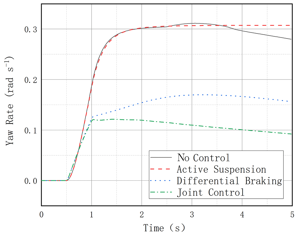
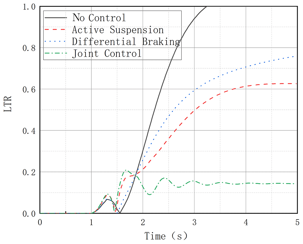
It can be seen that, without any control, the vehicle reaches the LTR value of 1 after 2.6 s, which means that the vehicle has experienced a rollover; all three control modes with control action have anti-rollover capability, and the joint control mode has the best anti-rollover effect with the smallest LTR value and slowly decreases due to the decrease in vehicle speed caused by differential braking. The differential braking mode and the active suspension control on their own are also effective in reducing the LTR value, as seen in Fig. 10. It can be seen that the uncontrolled vehicle roll angle value changes dramatically, reaching 30° in less than 2 s compared to the combined control vehicle roll angle, which fluctuates in the range of 0–2 (Fig. 11). In Fig. 12, the lateral acceleration comparison graph and the transverse sway angular velocity comparison graph both show that the joint control has a controlling effect on the lateral stability of the vehicle, which can also be seen in Fig. 13.

Figure 15 Roll angle.

Figure 16 Lateral acceleration.

Figure 17 Yaw rate.

4.2 Fishhook steering working condition

The dynamic rollover simulation test (fishhook steering test) was conducted under the road condition with an adhesion coefficient of 0.8. The vehicle speed was set to 60 km h⁻¹, the front-wheel turning angle was the fishhook turning angle, the starting time was 1s, the left turning angle was a positive maximum value of 2.5° and the right turning angle was a negative maximum value of −5°. The simulation results are shown in the figures. In Fig. 14, it can be seen that in the fishhook condition, the vehicle without control reaches the LTR value of 1 after 3.2 s; that is, the vehicle rolls over. Compared with the single control mode, joint control has a more significant effect in reducing the LTR value. Such characteristics can be seen in the sway angle (Fig. 15), lateral acceleration (Fig. 16) and transverse angular velocity (Fig. 17) as well, meaning that joint control is better than individual active suspension control and differential braking control, which have strong anti-rollover capability of the vehicle.

Figure 18 Step condition.

Figure 19 Fishhook condition.

4.3 Advantages of joint control

From the above simulation results and relevant literature, it can be explained that the single braking control and suspension control can improve the vehicle rollover dynamic characteristics to varying degrees, but they are not as effective as the joint control. Such problems come from the coupling characteristics of vehicle dynamics and tire force. We know that when the vehicle is rolling at a large angle, the vertical force of the tires on both sides of the wheel changes, and the braking wheels often cannot provide enough tire-braking force. Through active suspension control, we can improve the vertical force of the wheels on both sides of the vehicle and increase the value of the additional yaw moment. Figures 18 and 19 are the comparison diagrams of the actual additional yaw moment and the ideal yaw moment under the above two working conditions, with two control modes a nd separate differential braking and joint control. It can be seen that joint control can provide a greater additional yaw moment.

5 Conclusions

1. Tackling the problem of improving the operational stability of three-axis emergency rescue vehicles and reducing the risk of vehicle rollover, a comprehensive three-axle rescue vehicle rollover dynamics model, integrating active suspension and a nonlinear tire model, is developed in this paper.

2. Through consideration of vehicle dynamics and tire force coupling, an innovative joint control strategy was devised, harnessing the synergies of both differential braking and active suspension systems. This strategy aims to enhance anti-rollover capabilities.

3. Simulation comparisons in multiple control modes and under different operating conditions demonstrate that the proposed joint control strategy and integrated controller significantly improve the anti-rollover performance of the vehicle. The adaptive model predictive control (MPC) controller designed in this paper has shown good robustness and effectiveness in simulating the two rollover dynamics of a three-axle rescue vehicle based on a nonlinear tire model.

Appendix A

Matrix A1

$A_{\mathrm{1}}=\left[\begin{array}{cccccccccc}\mathrm{0}& \mathrm{1}& \mathrm{0}& \mathrm{0}& \mathrm{0}& \mathrm{0}& \mathrm{0}& \mathrm{0}& \mathrm{0}& \mathrm{0}\\ \frac{-\mathrm{6}{k}_s}{m_s}& \frac{-\mathrm{6}{c}_s}{m_s}& \frac{k_s}{m_s}& \frac{c_s}{m_s}& \frac{k_s}{m_s}& \frac{c_s}{m_s}& \frac{k_s}{m_s}& \frac{c_s}{m_s}& \frac{k_s}{m_s}& \frac{c_s}{m_s}\\ \mathrm{0}& \mathrm{0}& \mathrm{0}& \mathrm{1}& \mathrm{0}& \mathrm{0}& \mathrm{0}& \mathrm{0}& \mathrm{0}& \mathrm{0}\\ \frac{k_s}{m_u}& \frac{c_s}{m_u}& \frac{-\left(k_s+k_t\right)}{m_u}& \frac{-c_s}{m_s}& \mathrm{0}& \mathrm{0}& \mathrm{0}& \mathrm{0}& \mathrm{0}& \mathrm{0}\\ \mathrm{0}& \mathrm{0}& \mathrm{0}& \mathrm{0}& \mathrm{0}& \mathrm{1}& \mathrm{0}& \mathrm{0}& \mathrm{0}& \mathrm{0}\\ \frac{k_s}{m_u}& \frac{c_s}{m_u}& \mathrm{0}& \mathrm{0}& \frac{-\left(k_s+k_t\right)}{m_u}& \frac{-c_s}{m_s}& \mathrm{0}& \mathrm{0}& \mathrm{0}& \mathrm{0}\\ \mathrm{0}& \mathrm{0}& \mathrm{0}& \mathrm{0}& \mathrm{0}& \mathrm{0}& \mathrm{0}& \mathrm{1}& \mathrm{0}& \mathrm{0}\\ \frac{k_s}{m_u}& \frac{c_s}{m_u}& \mathrm{0}& \mathrm{0}& \mathrm{0}& \mathrm{0}& \frac{-\left(k_s+k_t\right)}{m_u}& \frac{-c_s}{m_u}& \mathrm{0}& \mathrm{0}\\ \mathrm{0}& \mathrm{0}& \mathrm{0}& \mathrm{0}& \mathrm{0}& \mathrm{0}& \mathrm{0}& \mathrm{0}& \mathrm{0}& \mathrm{1}\\ \frac{k_s}{m_u}& \frac{c_s}{m_u}& \mathrm{0}& \mathrm{0}& \mathrm{0}& \mathrm{0}& \mathrm{0}& \mathrm{0}& \frac{-\left(k_s+k_t\right)}{m_u}& \frac{-c_s}{m_u}\\ \mathrm{0}& \mathrm{0}& \mathrm{0}& \mathrm{0}& \mathrm{0}& \mathrm{0}& \mathrm{0}& \mathrm{0}& \mathrm{0}& \mathrm{0}\\ \frac{k_s}{m_u}& \frac{c_s}{m_u}& \mathrm{0}& \mathrm{0}& \mathrm{0}& \mathrm{0}& \mathrm{0}& \mathrm{0}& \mathrm{0}& \mathrm{0}\\ \mathrm{0}& \mathrm{0}& \mathrm{0}& \mathrm{0}& \mathrm{0}& \mathrm{0}& \mathrm{0}& \mathrm{0}& \mathrm{0}& \mathrm{0}\\ \frac{k_s}{m_u}& \frac{c_s}{m_u}& \mathrm{0}& \mathrm{0}& \mathrm{0}& \mathrm{0}& \mathrm{0}& \mathrm{0}& \mathrm{0}& \mathrm{0}\\ \mathrm{0}& \mathrm{0}& \mathrm{0}& \mathrm{0}& \mathrm{0}& \mathrm{0}& \mathrm{0}& \mathrm{0}& \mathrm{0}& \mathrm{0}\\ \frac{\mathrm{2}{l}_{\mathrm{1}}{k}_s-\mathrm{2}{l}_{\mathbf{2}}{k}_s-\mathrm{2}{l}_{\mathbf{3}}{k}_s}{I_y}& \frac{\mathrm{2}{l}_{\mathrm{1}}{c}_s-\mathrm{2}{l}_{\mathbf{2}}{c}_s-\mathrm{2}{l}_{\mathbf{3}}{c}_s}{I_y}& \frac{-l_{\mathrm{1}}{k}_s}{I_y}& \frac{-l_{\mathrm{1}}{c}_s}{I_y}& \frac{-l_{\mathrm{1}}{k}_s}{I_y}& \frac{-l_{\mathrm{1}}{c}_s}{I_y}& \frac{l_{\mathrm{1}}{k}_s}{I_y}& \frac{l_{\mathrm{1}}{c}_s}{I_y}& \frac{l_{\mathbf{2}}{k}_s}{I_y}& \frac{l_{\mathbf{2}}{c}_s}{I_y}\\ \mathrm{0}& \mathrm{0}& \mathrm{0}& \mathrm{0}& \mathrm{0}& \mathrm{0}& \mathrm{0}& \mathrm{0}& \mathrm{0}& \mathrm{0}\\ \mathrm{0}& \mathrm{0}& \frac{m{b}_{\mathrm{1}}{k}_s}{\mathrm{2}\left(m{I}_x-m_s^{\mathrm{2}}{h}_s^{\mathrm{2}}\right)}& \frac{m{b}_{\mathrm{1}}{c}_s}{\mathrm{2}\left(m{I}_x-m_s^{\mathrm{2}}{h}_s^{\mathrm{2}}\right)}& \frac{-m{b}_{\mathrm{1}}{k}_s}{\mathrm{2}\left(m{I}_x-m_s^{\mathrm{2}}{h}_s^{\mathrm{2}}\right)}& \frac{-m{b}_{\mathrm{1}}{c}_s}{\mathrm{2}\left(m{I}_x-m_s^{\mathrm{2}}{h}_s^{\mathrm{2}}\right)}& \frac{m{b}_{\mathrm{2}}{k}_s}{\mathrm{2}\left(m{I}_x-m_s^{\mathrm{2}}{h}_s^{\mathrm{2}}\right)}& \frac{m{b}_{\mathrm{2}}{c}_s}{\mathrm{2}\left(m{I}_x-m_s^{\mathrm{2}}{h}_s^{\mathrm{2}}\right)}& \frac{-m{b}_{\mathrm{2}}{k}_s}{\mathrm{2}\left(m{I}_x-m_s^{\mathrm{2}}{h}_s^{\mathrm{2}}\right)}& \frac{-m{b}_{\mathrm{2}}{c}_s}{\mathrm{2}\left(m{I}_x-m_s^{\mathrm{2}}{h}_s^{\mathrm{2}}\right)}\\ \mathrm{0}& \mathrm{0}& \frac{m_s{b}_{\mathrm{1}}{h}_s{k}_s}{\mathrm{2}v\left(m{I}_x-m_s^{\mathrm{2}}{h}_s^{\mathrm{2}}\right)}& \frac{m_s{b}_{\mathrm{1}}{h}_s{c}_s}{\mathrm{2}v\left(m{I}_x-m_s^{\mathrm{2}}{h}_s^{\mathrm{2}}\right)}& \frac{-m_s{b}_{\mathrm{1}}{h}_s{k}_s}{\mathrm{2}v\left(m{I}_x-m_s^{\mathrm{2}}{h}_s^{\mathrm{2}}\right)}& \frac{-m_s{b}_{\mathrm{1}}{h}_s{c}_s}{\mathrm{2}v\left(m{I}_x-m_s^{\mathrm{2}}{h}_s^{\mathrm{2}}\right)}& \frac{m_s{b}_{\mathrm{2}}{h}_s{k}_s}{\mathrm{2}v\left(m{I}_x-m_s^{\mathrm{2}}{h}_s^{\mathrm{2}}\right)}& \frac{m_s{b}_{\mathrm{2}}{h}_s{c}_s}{\mathrm{2}v\left(m{I}_x-m_s^{\mathrm{2}}{h}_s^{\mathrm{2}}\right)}& \frac{-m_s{b}_{\mathrm{2}}{h}_s{k}_s}{\mathrm{2}v\left(m{I}_x-m_s^{\mathrm{2}}{h}_s^{\mathrm{2}}\right)}& \frac{-m_s{b}_{\mathrm{2}}{h}_s{c}_s}{\mathrm{2}v\left(m{I}_x-m_s^{\mathrm{2}}{h}_s^{\mathrm{2}}\right)}\\ \mathrm{0}& \mathrm{0}& \mathrm{0}& \mathrm{0}& \mathrm{0}& \mathrm{0}& \mathrm{0}& \mathrm{0}& \mathrm{0}& \mathrm{0}\end{array}\right]$

Matrix A2

$${\displaystyle }{A}_{\mathrm{2}}=\left[\begin{array}{cccccccccc}\mathrm{0}& \mathrm{1}& \mathrm{0}& \mathrm{0}& \mathrm{0}& \mathrm{0}& \mathrm{0}& \mathrm{0}& \mathrm{0}& \mathrm{0}\\ \frac{k_{s\mathrm{31}}}{m_s}& \frac{c_{s\mathrm{31}}}{m_s}& \frac{k_{s\mathrm{32}}}{m_s}& \frac{c_{s\mathrm{32}}}{m_s}& a_{\mathrm{2},\mathrm{15}}& a_{\mathrm{2},\mathrm{16}}& \mathrm{0}& \mathrm{0}& \mathrm{0}& \mathrm{0}\\ \mathrm{0}& \mathrm{0}& \mathrm{0}& \mathrm{0}& \mathrm{0}& \mathrm{0}& \mathrm{0}& \mathrm{0}& \mathrm{0}& \mathrm{0}\\ \mathrm{0}& \mathrm{0}& \mathrm{0}& \mathrm{0}& \frac{-k_{s\mathrm{11}}{l}_{\mathrm{1}}}{m_{u\mathrm{11}}}& \frac{-c_{s\mathrm{11}}{l}_{\mathrm{1}}}{m_{u\mathrm{11}}}& \frac{k_{s\mathrm{11}}{b}_{\mathrm{1}}}{\mathrm{2}{m}_{u\mathrm{11}}}& \frac{c_{s\mathrm{11}}{b}_{\mathrm{1}}}{\mathrm{2}{m}_{u\mathrm{11}}}& \mathrm{0}& \mathrm{0}\\ \mathrm{0}& \mathrm{0}& \mathrm{0}& \mathrm{0}& \mathrm{0}& \mathrm{0}& \mathrm{0}& \mathrm{0}& \mathrm{0}& \mathrm{0}\\ \mathrm{0}& \mathrm{0}& \mathrm{0}& \mathrm{0}& \frac{-k_{s\mathrm{12}}{l}_{\mathrm{1}}}{m_{u\mathrm{12}}}& \frac{-c_{s\mathrm{12}}{l}_{\mathrm{1}}}{m_{u\mathrm{12}}}& \frac{-k_{s\mathrm{12}}{b}_{\mathrm{1}}}{\mathrm{2}{m}_{u\mathrm{12}}}& \frac{-c_{s\mathrm{12}}{b}_{\mathrm{1}}}{\mathrm{2}{m}_{u\mathrm{12}}}& \mathrm{0}& \mathrm{0}\\ \mathrm{0}& \mathrm{0}& \mathrm{0}& \mathrm{0}& \mathrm{0}& \mathrm{0}& \mathrm{0}& \mathrm{1}& \mathrm{0}& \mathrm{0}\\ \mathrm{0}& \mathrm{0}& \mathrm{0}& \mathrm{0}& \frac{k_{s\mathrm{21}}{l}_{\mathrm{2}}}{m_{u\mathrm{21}}}& \frac{c_{s\mathrm{21}}{l}_{\mathrm{2}}}{m_{u\mathrm{21}}}& \frac{k_{s\mathrm{21}}{b}_{\mathrm{2}}}{\mathrm{2}{m}_{u\mathrm{21}}}& \frac{c_{s\mathrm{21}}{b}_{\mathrm{2}}}{\mathrm{2}{m}_{u\mathrm{11}}}& \mathrm{0}& \mathrm{0}\\ \mathrm{0}& \mathrm{0}& \mathrm{0}& \mathrm{0}& \mathrm{0}& \mathrm{0}& \mathrm{0}& \mathrm{0}& \mathrm{0}& \mathrm{0}\\ \mathrm{0}& \mathrm{0}& \mathrm{0}& \mathrm{0}& \frac{k_{s\mathrm{22}}{l}_{\mathrm{2}}}{m_{u\mathrm{22}}}& \frac{c_{s\mathrm{22}}{l}_{\mathrm{2}}}{m_{u\mathrm{22}}}& \frac{-k_{s\mathrm{22}}{b}_{\mathrm{2}}}{\mathrm{2}{m}_{u\mathrm{22}}}& \frac{-c_{s\mathrm{22}}{b}_{\mathrm{2}}}{\mathrm{2}{m}_{u\mathrm{22}}}& \mathrm{0}& \mathrm{0}\\ \mathrm{0}& \mathrm{1}& \mathrm{0}& \mathrm{0}& \mathrm{0}& \mathrm{0}& \mathrm{0}& \mathrm{0}& \mathrm{0}& \mathrm{0}\\ \frac{-\left(k_{s\mathrm{31}}+k_t\right)}{m_{u\mathrm{31}}}& \frac{-c_{s\mathrm{31}}}{m_{u\mathrm{31}}}& \mathrm{0}& \mathrm{0}& \frac{k_{s\mathrm{31}}{l}_{\mathrm{3}}}{m_{u\mathrm{31}}}& \frac{c_{s\mathrm{31}}{l}_{\mathrm{3}}}{m_{u\mathrm{31}}}& \frac{k_{s\mathrm{31}}{b}_{\mathrm{3}}}{\mathrm{2}{m}_{u\mathrm{31}}}& \frac{c_{s\mathrm{31}}{b}_{\mathrm{3}}}{\mathrm{2}{m}_{u\mathrm{31}}}& \mathrm{0}& \mathrm{0}\\ \mathrm{0}& \mathrm{0}& \mathrm{0}& \mathrm{1}& \mathrm{0}& \mathrm{0}& \mathrm{0}& \mathrm{0}& \mathrm{0}& \mathrm{0}\\ \mathrm{0}& \mathrm{0}& \frac{-\left(k_{s\mathrm{32}}+k_t\right)}{m_{u\mathrm{32}}}& \frac{-c_{s\mathrm{32}}}{m_{u\mathrm{32}}}& \frac{k_{s\mathrm{32}}{l}_{\mathrm{3}}}{m_{u\mathrm{32}}}& \frac{c_{s\mathrm{32}}{l}_{\mathrm{3}}}{m_{u\mathrm{32}}}& \frac{-k_{s\mathrm{32}}{b}_{\mathrm{3}}}{\mathrm{2}{m}_{u\mathrm{32}}}& \frac{-c_{s\mathrm{32}}{b}_{\mathrm{3}}}{\mathrm{2}{m}_{u\mathrm{32}}}& \mathrm{0}& \mathrm{0}\\ \mathrm{0}& \mathrm{0}& \mathrm{0}& \mathrm{0}& \mathrm{0}& \mathrm{1}& \mathrm{0}& \mathrm{0}& \mathrm{0}& \mathrm{0}\\ \frac{l_{\mathbf{3}}{k}_{s\mathrm{31}}}{I_y}& \frac{l_{\mathbf{3}}{c}_{s\mathrm{31}}}{I_y}& \frac{l_{\mathbf{3}}{k}_{s\mathrm{32}}}{I_y}& \frac{l_{\mathbf{2}}{c}_{s\mathrm{32}}}{I_y}& a_{\mathrm{16},\mathrm{15}}& a_{\mathrm{16},\mathrm{16}}& \mathrm{0}& \mathrm{0}& \mathrm{0}& \mathrm{0}\\ \mathrm{0}& \mathrm{0}& \mathrm{0}& \mathrm{0}& \mathrm{0}& \mathrm{0}& \mathrm{0}& \mathrm{1}& \mathrm{0}& \mathrm{0}\\ \frac{-m{b}_{\mathrm{2}}{k}_{s\mathrm{22}}}{\mathrm{2}\left(m{I}_x-m_s^{\mathrm{2}}{h}_s^{\mathrm{2}}\right)}& \frac{-m{b}_{\mathrm{2}}{c}_{s\mathrm{22}}}{\mathrm{2}\left(m{I}_x-m_s^{\mathrm{2}}{h}_s^{\mathrm{2}}\right)}& \frac{m{b}_{\mathrm{3}}{k}_{s\mathrm{31}}}{\mathrm{2}\left(m{I}_x-m_s^{\mathrm{2}}{h}_s^{\mathrm{2}}\right)}& \frac{m{b}_{\mathrm{3}}{c}_{s\mathrm{31}}}{\mathrm{2}\left(m{I}_x-m_s^{\mathrm{2}}{h}_s^{\mathrm{2}}\right)}& \mathrm{0}& \mathrm{0}& a_{\mathrm{18},\mathrm{15}}& a_{\mathrm{18},\mathrm{16}}& a_{\mathrm{18},\mathrm{17}}& a_{\mathrm{18},\mathrm{18}}\\ \frac{k_{s\mathrm{31}}{b}_{\mathrm{3}}{m}_s{h}_s}{\mathrm{2}v\left(m{I}_x-m_s^{\mathrm{2}}{h}_s^{\mathrm{2}}\right)}& \frac{c_{s\mathrm{31}}{b}_{\mathrm{3}}{m}_s{h}_s}{\mathrm{2}v\left(m{I}_x-m_s^{\mathrm{2}}{h}_s^{\mathrm{2}}\right)}& \frac{-k_{s\mathrm{32}}{b}_{\mathrm{3}}{m}_s{h}_s}{\mathrm{2}v\left(m{I}_x-m_s^{\mathrm{2}}{h}_s^{\mathrm{2}}\right)}& \frac{-c_{s\mathrm{32}}{b}_{\mathrm{3}}{m}_s{h}_s}{\mathrm{2}v\left(m{I}_x-m_s^{\mathrm{2}}{h}_s^{\mathrm{2}}\right)}& \mathrm{0}& \mathrm{0}& a_{\mathrm{19},\mathrm{17}}& a_{\mathrm{19},\mathrm{18}}& a_{\mathrm{19},\mathrm{19}}& a_{\mathrm{19},\mathrm{20}}\\ \mathrm{0}& \mathrm{0}& \mathrm{0}& \mathrm{0}& \mathrm{0}& \mathrm{0}& \mathrm{0}& \mathrm{0}& a_{\mathrm{20},\mathrm{19}}& a_{\mathrm{20},\mathrm{20}}\end{array}\right]$$

In the matrix, the values are as follows: $a_{\mathrm{2},\mathrm{15}}=\frac{\mathrm{2}{l}_{\mathrm{1}}{k}_s-\mathrm{2}{l}_{\mathrm{2}}{k}_s-\mathrm{2}{l}_{\mathrm{3}}{k}_s}{m_s}$, $a_{\mathrm{2},\mathrm{16}}=\frac{\mathrm{2}{l}_{\mathrm{1}}{c}_s-\mathrm{2}{l}_{\mathrm{2}}{c}_s-\mathrm{2}{l}_{\mathrm{3}}{c}_s}{m_s}$, $a_{\mathrm{16},\mathrm{15}}=\frac{-\mathrm{2}{k}_s(l_{\mathrm{1}}^{\mathrm{2}}+l_{\mathrm{2}}^{\mathrm{2}}+l_{\mathrm{3}}^{\mathrm{2}})}{I_y}+\frac{m_{s}hg}{I_y}$, $a_{\mathrm{16},\mathrm{16}}=\frac{-\mathrm{2}{c}_s(l_{\mathrm{1}}^{\mathrm{2}}+l_{\mathrm{2}}^{\mathrm{2}}+l_{\mathrm{3}}^{\mathrm{2}})}{I_y}$, $a_{\mathrm{18},\mathrm{15}}=\frac{-\mathrm{3}m{k}_s{l}_w^{\mathrm{2}}}{\mathrm{2}(m{I}_x-m_s^{\mathrm{2}}{h}^{\mathrm{2}})}+\frac{m{m}_{s}hg}{m{I}_x-m_s^{\mathrm{2}}{h}^{\mathrm{2}}}$, $a_{\mathrm{18},\mathrm{16}}=\frac{-\mathrm{3}{c}_{s}m{l}_w^{\mathrm{2}}}{\mathrm{2}(m{I}_x-m_s^{\mathrm{2}}{h}^{\mathrm{2}})}$, $a_{\mathrm{18},\mathrm{17}}=\frac{\mathrm{6}{k}_t{m}_{s}h}{m{I}_x-m_s^{\mathrm{2}}{h}^{\mathrm{2}}}$, $a_{\mathrm{18},\mathrm{18}}=\frac{\mathrm{2}{k}_t(l_{\mathrm{1}}-l_{\mathrm{2}}-l_{\mathrm{3}})m_{s}h}{v(m{I}_x-m_s^{\mathrm{2}}{h}^{\mathrm{2}})}$, $a_{\mathrm{19},\mathrm{17}}=\frac{-\mathrm{3}{k}_s{m}_s{l}_w^{\mathrm{2}}h}{\mathrm{2}v(m{I}_x-m_s^{\mathrm{2}}{h}^{\mathrm{2}})}+\frac{m_s^{\mathrm{2}}{h}^{\mathrm{2}}g}{v(m{I}_x-m_s^{\mathrm{2}}{h}^{\mathrm{2}})}$, $a_{\mathrm{19},\mathrm{18}}=\frac{-\mathrm{3}{c}_s{m}_s{l}_w^{\mathrm{2}}h}{\mathrm{2}v(m{I}_x-m_s^{\mathrm{2}}{h}^{\mathrm{2}})}$, $a_{\mathrm{19},\mathrm{19}}=\frac{\mathrm{6}{k}_t{I}_x}{v(m{I}_x-m_s^{\mathrm{2}}{h}^{\mathrm{2}})}$, $a_{\mathrm{19},\mathrm{20}}=\frac{\mathrm{2}{I}_x{k}_t(l_{\mathrm{1}}-l_{\mathrm{2}}-l_{\mathrm{3}})}{v^{\mathrm{2}}(m{I}_x-m_s^{\mathrm{2}}{h}^{\mathrm{2}})}-\mathrm{1}$, $a_{\mathrm{20},\mathrm{19}}=\frac{\mathrm{2}{k}_t(l_{\mathrm{1}}-l_{\mathrm{2}}-l_{\mathrm{3}})}{I_z}$ and $a_{\mathrm{20},\mathrm{20}}=\frac{\mathrm{2}{k}_t(l_{\mathrm{1}}^{\mathrm{2}}+l_{\mathrm{2}}^{\mathrm{2}}+l_{\mathrm{3}}^{\mathrm{2}})}{I_{z}v}$.

Appendix B

Matrix B1

$${\displaystyle }{B}_{\mathrm{1}}=\left[\begin{array}{cccccccc}\mathrm{0}& \mathrm{0}& \mathrm{0}& \mathrm{0}& \mathrm{0}& \mathrm{0}& \mathrm{0}& \mathrm{0}\\ \mathrm{0}& \mathrm{0}& \frac{\mathrm{1}}{m_s}& \frac{\mathrm{1}}{m_s}& \frac{\mathrm{1}}{m_s}& \frac{\mathrm{1}}{m_s}& \frac{\mathrm{1}}{m_s}& \frac{\mathrm{1}}{m_s}\\ \mathrm{0}& \mathrm{0}& \mathrm{0}& \mathrm{0}& \mathrm{0}& \mathrm{0}& \mathrm{0}& \mathrm{0}\\ \mathrm{0}& \mathrm{0}& \frac{-\mathrm{1}}{m_{u\mathrm{11}}}& \mathrm{0}& \mathrm{0}& \mathrm{0}& \mathrm{0}& \mathrm{0}\\ \mathrm{0}& \mathrm{0}& \mathrm{0}& \mathrm{0}& \mathrm{0}& \mathrm{0}& \mathrm{0}& \mathrm{0}\\ \mathrm{0}& \mathrm{0}& \mathrm{0}& \frac{-\mathrm{1}}{m_{u\mathrm{12}}}& \mathrm{0}& \mathrm{0}& \mathrm{0}& \mathrm{0}\\ \mathrm{0}& \mathrm{0}& \mathrm{0}& \mathrm{0}& \mathrm{0}& \mathrm{0}& \mathrm{0}& \mathrm{1}\\ \mathrm{0}& \mathrm{0}& \mathrm{0}& \mathrm{0}& \frac{-\mathrm{1}}{m_{u\mathrm{21}}}& \mathrm{0}& \mathrm{0}& \mathrm{0}\\ \mathrm{0}& \mathrm{0}& \mathrm{0}& \mathrm{0}& \mathrm{0}& \mathrm{0}& \mathrm{0}& \mathrm{0}\\ \mathrm{0}& \mathrm{0}& \mathrm{0}& \mathrm{0}& \mathrm{0}& \frac{-\mathrm{1}}{m_{u\mathrm{22}}}& \mathrm{0}& \mathrm{0}\\ \mathrm{0}& \mathrm{0}& \mathrm{0}& \mathrm{0}& \mathrm{0}& \mathrm{0}& \mathrm{0}& \mathrm{0}\\ \mathrm{0}& \mathrm{0}& \mathrm{0}& \mathrm{0}& \mathrm{0}& \mathrm{0}& \frac{-\mathrm{1}}{m_{u\mathrm{31}}}& \mathrm{0}\\ \mathrm{0}& \mathrm{0}& \mathrm{0}& \mathrm{0}& \mathrm{0}& \mathrm{0}& \mathrm{0}& \mathrm{0}\\ \mathrm{0}& \mathrm{0}& \mathrm{0}& \mathrm{0}& \mathrm{0}& \mathrm{0}& \mathrm{0}& \frac{-\mathrm{1}}{m_{u\mathrm{32}}}\\ \mathrm{0}& \mathrm{0}& \mathrm{0}& \mathrm{0}& \mathrm{0}& \mathrm{0}& \mathrm{0}& \mathrm{0}\\ \mathrm{0}& \mathrm{0}& \frac{-l_{\mathbf{1}}}{I_y}& \frac{-l_{\mathbf{1}}}{I_y}& \frac{-l_{\mathrm{2}}}{I_y}& \frac{-l_{\mathrm{2}}}{I_y}& \frac{-l_{\mathbf{3}}}{I_y}& \frac{-l_{\mathbf{3}}}{I_y}\\ \mathrm{0}& \mathrm{0}& \mathrm{0}& \mathrm{0}& \mathrm{0}& \mathrm{0}& \mathrm{0}& \mathrm{1}\\ \frac{-\mathrm{2}{k}_{\mathrm{1}}{m}_{s}h}{\left(m{I}_x-m_s^{\mathrm{2}}{h}_s^{\mathrm{2}}\right)}& \mathrm{0}& \frac{m{b}_{\mathrm{1}}}{\mathrm{2}\left(m{I}_x-m_s^{\mathrm{2}}{h}_s^{\mathrm{2}}\right)}& \frac{-m{b}_{\mathrm{1}}}{\mathrm{2}\left(m{I}_x-m_s^{\mathrm{2}}{h}_s^{\mathrm{2}}\right)}& \frac{m{b}_{\mathrm{2}}}{\mathrm{2}\left(m{I}_x-m_s^{\mathrm{2}}{h}_s^{\mathrm{2}}\right)}& \frac{-m{b}_{\mathrm{2}}}{\mathrm{2}\left(m{I}_x-m_s^{\mathrm{2}}{h}_s^{\mathrm{2}}\right)}& \frac{m{b}_{\mathrm{3}}}{\mathrm{2}\left(m{I}_x-m_s^{\mathrm{2}}{h}_s^{\mathrm{2}}\right)}& \frac{-m{b}_{\mathrm{3}}}{\mathrm{2}\left(m{I}_x-m_s^{\mathrm{2}}{h}_s^{\mathrm{2}}\right)}\\ \frac{-\mathrm{2}{k}_{\mathrm{1}}{I}_x}{v\left(m{I}_x-m_s^{\mathrm{2}}{h}_s^{\mathrm{2}}\right)}& \mathrm{0}& \frac{m_s{h}_s{b}_{\mathrm{1}}}{\mathrm{2}v\left(m{I}_x-m_s^{\mathrm{2}}{h}_s^{\mathrm{2}}\right)}& \frac{-m_s{h}_s{b}_{\mathrm{1}}}{\mathrm{2}v\left(m{I}_x-m_s^{\mathrm{2}}{h}_s^{\mathrm{2}}\right)}& \frac{m_s{h}_s{b}_{\mathrm{2}}}{\mathrm{2}v\left(m{I}_x-m_s^{\mathrm{2}}{h}_s^{\mathrm{2}}\right)}& \frac{-m_s{h}_s{b}_{\mathrm{2}}}{\mathrm{2}v\left(m{I}_x-m_s^{\mathrm{2}}{h}_s^{\mathrm{2}}\right)}& \frac{m_s{h}_s{b}_{\mathrm{3}}}{\mathrm{2}v\left(m{I}_x-m_s^{\mathrm{2}}{h}_s^{\mathrm{2}}\right)}& \frac{-m_s{h}_s{b}_{\mathrm{3}}}{\mathrm{2}v\left(m{I}_x-m_s^{\mathrm{2}}{h}_s^{\mathrm{2}}\right)}\\ \frac{-\mathrm{2}{l}_{\mathbf{1}}{k}_{\mathrm{1}}}{I_z}& \frac{\mathrm{1}}{I_z}& \mathrm{0}& \mathrm{0}& \mathrm{0}& \mathrm{0}& \mathrm{0}& \mathrm{0}\end{array}\right]$$

Matrix B2

$${\displaystyle }{B}_{\mathrm{2}}=\left[\begin{array}{cccccc}\mathrm{0}& \mathrm{0}& \mathrm{0}& \mathrm{0}& \mathrm{0}& \mathrm{0}\\ \mathrm{0}& \mathrm{0}& \mathrm{0}& \mathrm{0}& \mathrm{0}& \mathrm{0}\\ \mathrm{0}& \mathrm{0}& \mathrm{0}& \mathrm{0}& \mathrm{0}& \mathrm{0}\\ \frac{k_t}{m_{u\mathrm{11}}}& \mathrm{0}& \mathrm{0}& \mathrm{0}& \mathrm{0}& \mathrm{0}\\ \mathrm{0}& \mathrm{0}& \mathrm{0}& \mathrm{0}& \mathrm{0}& \mathrm{0}\\ \mathrm{0}& \frac{k_t}{m_{u\mathrm{12}}}& \mathrm{0}& \mathrm{0}& \mathrm{0}& \mathrm{0}\\ \mathrm{0}& \mathrm{0}& \mathrm{0}& \mathrm{0}& \mathrm{0}& \mathrm{0}\\ \mathrm{0}& \mathrm{0}& \frac{k_t}{m_{u\mathrm{21}}}& \mathrm{0}& \mathrm{0}& \mathrm{0}\\ \mathrm{0}& \mathrm{0}& \mathrm{0}& \mathrm{0}& \mathrm{0}& \mathrm{0}\\ \mathrm{0}& \mathrm{0}& \mathrm{0}& \frac{k_t}{m_{u\mathrm{22}}}& \mathrm{0}& \mathrm{0}\\ \mathrm{0}& \mathrm{0}& \mathrm{0}& \mathrm{0}& \mathrm{0}& \mathrm{0}\\ \mathrm{0}& \mathrm{0}& \mathrm{0}& \mathrm{0}& \frac{k_t}{m_{u\mathrm{31}}}& \mathrm{0}\\ \mathrm{0}& \mathrm{0}& \mathrm{0}& \mathrm{0}& \mathrm{0}& \mathrm{0}\\ \mathrm{0}& \mathrm{0}& \mathrm{0}& \mathrm{0}& \mathrm{0}& \frac{k_t}{m_{u\mathrm{32}}}\\ \mathrm{0}& \mathrm{0}& \mathrm{0}& \mathrm{0}& \mathrm{0}& \mathrm{0}\\ \mathrm{0}& \mathrm{0}& \mathrm{0}& \mathrm{0}& \mathrm{0}& \mathrm{0}\\ \mathrm{0}& \mathrm{0}& \mathrm{0}& \mathrm{0}& \mathrm{0}& \mathrm{0}\\ \mathrm{0}& \mathrm{0}& \mathrm{0}& \mathrm{0}& \mathrm{0}& \mathrm{0}\\ \mathrm{0}& \mathrm{0}& \mathrm{0}& \mathrm{0}& \mathrm{0}& \mathrm{0}\\ \mathrm{0}& \mathrm{0}& \mathrm{0}& \mathrm{0}& \mathrm{0}& \mathrm{0}\end{array}\right]$$

Appendix C

$b_{\mathrm{1},\mathrm{2},\mathrm{3}}$	wheelbase of each axle
cs	suspension damping
Fyij	lateral tire force of each wheel, where $i=\mathrm{1},\mathrm{2},\mathrm{3}$
	represents the front, middle and rear axles
	and $j=\mathrm{1},\mathrm{2}$ represents left and right
Ftij	vertical tire force of each wheel
Fij	vertical suspension force of each wheel
fij	actuation force of each wheel's active
	suspension actuator
g	gravity acceleration
hs	distance from sprung mass center of gravity
	to roll center
$I_{xx,yy,zz}$	moment of inertia of the respective axle
kt	tire vertical stiffness
$l_{\mathrm{1},\mathrm{2},\mathrm{3}}$	distance from center of gravity to
	front, middle or rear axle
m	vehicle mass
ms	vehicle sprung mass
muij	suspension and tire mass
zm	vehicle centroid displacement
zsij	displacement of the body on the suspension
zuij	displacement of the wheels
zrij	road excitation of each tire
v	vehicle's longitudinal velocity
β	vehicle body sideslip angle
ω	yaw angle rate
θ	pitch angle
φ	roll angle
δ	steering-wheel angle
wz	additional yaw moment