Design and error compensation of a 3-degrees-of-freedom cable-driven hybrid 3D-printing mechanism

In large-scale 3D additive manufacturing (AM), rigid printing mechanisms exhibit high inertia and inadequate load capacity. In this paper, a fully constrained 3-degrees-of-freedom (DOFs) cable-driven hybrid mechanism (CDHR) is developed. A vector analysis method considering error compensation in the pulley system is proposed for analysing the kinematics and dynamics. To address the cable-driven mechanism's strict cable force range requirement, a prescribed-performance controller (PPC) with an adaptive auxiliary system is designed for the nonlinear cable system to enhance the stability and motion accuracy of the end-effector. The stability of the control system is proven using the Lyapunov function. A physical simulation environment using Simscape is developed to verify the vector analysis method and the PPC. Subsequently, an experimental prototype of a 3-DOF CDHR is developed. The results of the error compensation experiment and the prescribed-performance controller experiment demonstrate a 93.321 % reduction in maximum plane error and a 95.376 % reduction in maximum height error for the PPC considering error compensation compared to the non-compensation trajectory. Finally, a double-layer clay-printing experiment is conducted to validate the feasibility of the mechanism.

1 Introduction

Cable-driven mechanisms have been widely used in the construction industry, haptic interactive robots, winding hoists, rehabilitation robots, aerospace, underwater manipulators, and other fields (Breseghello and Naboni, 2022; Song et al., 2023; Ding et al., 2022; Ben Hamida et al., 2021; Amin et al., 2020; Yang et al., 2023; Xue and Fan, 2022). In large-scale 3D additive manufacturing, rigid printing mechanisms suffer from high inertia and inadequate load capacity. The cable-driven 3D-printing mechanism replaces rigid links with flexible cables to solve these problems. The cable-driven parallel mechanism can possess the characteristics of a parallel mechanism, such as high precision, no error accumulation, and rapid dynamic response, while also increasing the working space, load capacity, and reconfigurability of the mechanism. Research on cable-driven mechanisms in mechanism design, cable force analysis, and motion control is gradually increasing to meet the requirements of additive manufacturing.

In the mechanism design of cable-driven parallel robots (CDPRs), Verhoeven et al. (1998) classified CDPRs into three types: under-constrained, fully constrained, and redundantly constrained mechanisms based on the relationship between the number of end-effector degrees of freedom (DOFs) and the number of driven cables. Bosscher et al. (2007) proposed a 3D-printing CDPR. Barnett and Gosselin (2015) designed a 6-DOF CDPR 3D printer and printed a 2160 mm statue using polyurethane foam. Jung (2020) proposed a CDPR with a retractable end-effector, which effectively improve the working space. Zhang et al. (2021) proposed a redundantly constrained CDPR for lunar 3D printing. The mechanism has eight winding pulleys in the same plane. Four cables connect to the end-effector attachment points in the upper part of the end-effector, and the remaining four cables connect to the lower part of the end-effector. The mechanism can operate stably under low gravity. Lee and Gwak (2022) proposed a redundantly constrained cable-driven mechanism for architectural 3D printing using four vertical moving elements with five cables. Nguyen-Van and Gwak (2022) proposed a CDPR with two nozzles to improve the printing efficiency. Alikhani et al. (2009) proposed a CDPR with nine cables controlling the end-effector based on the principle of the parallelogram. The mechanism requires only three motors to control the 3 DOFs of the end-effector. In the error analysis and compensation of the cable-driven mechanism, Izard et al. (2017) used the 6-DOF redundant cable-driven mechanism to analyse the printing error and the influence of the printing trajectory on the printing accuracy. Gueners et al. (2022) used a redundant cable-driven mechanism with eight cables to control the 6-DOF end-effector. A radial cable-winding system is proposed to improve the precision of cable winding. Tho and Thinh (2021) used the trust-region-dogleg equation to analyse the cable and improve the accuracy of kinematics analysis.

All of the mechanisms mentioned above are redundantly constrained mechanisms. Most of these mechanisms achieve unidirectional force transmission by applying mutual pulls between the cables. However, this approach significantly reduces the efficiency of the cable-driven mechanism and increases the complexity of cable force analysis and motion control. Consequently, the approach of incorporating springs in cable-driven mechanisms to maintain cable tension has been widely adopted. Russell (1994) proposed the utilization of springs to regulate cable forces in CDPRs, with the additional function of providing overload protection. Trevisani (2010) employed torsion springs to ensure the tension in a planar flexure parallel mechanism. Jung and Bae (2016) integrated springs into a cable-driven mechanism to enhance the unidirectional force characteristics of the cables, enabling them to transmit forces in two directions. Perreault et al. (2014) explored the approach of distributing cable forces in a spring-loaded cable-driven mechanism. Taghavi et al. (2013) demonstrated that incorporating springs can expand the working space of a multi-body cable-driven robot. Zi et al. (2019) and Qian et al. (2018) proposed a fully constrained cable-driven mechanism that utilizes six cables and a spring, significantly reducing the complexity of cable force analysis and motion control. Duan et al. (2022) proposed the Tbot robot, which replaces the rigid links of the Delta robot with cables. This mechanism incorporates a spring-loaded link to ensure proper cable tension and to enable high-speed motion of the end-effector.

Due to the strict cable force range requirement of the cable-driven mechanism, the introduction of springs introduces additional uncertainty to the mechanism. Consequently, controller design is commonly employed to minimize end-effector motion error and to improve the stability of the mechanism. Jiang et al. (2017) utilized springs to ensure tension in three cables, developed a spring dynamics model, and designed controllers using linear quadratic optimal control (LQOC). Fang et al. (2021) analysed various controller types commonly employed in CDPRs, including impedance-based, proportional–integral–derivative (PID)-based, admittance-based, assist-as-needed (AAN), and adaptive controllers. Song and Lau (2022) proposed a workspace-based model-predictive-control method for addressing the unidirectional force characteristics of cables in redundant cable-driven mechanisms. Xie et al. (2021) proposed the coordinated dynamic control in the task space (CDCT) for a cable-driven parallel redundant robot, which ensures high tracking accuracy. The controller's robustness is analysed, and the stability of the control system is demonstrated. All of the aforementioned controllers ensure the fulfilment of unidirectional force transmission characteristics in the cables.

The accuracy of moulded parts in additive manufacturing methods, such as fused deposition modelling (FDM), stereolithography apparatus (SLA), and selective laser melting (SLM), primarily relies on the precise movement of the x axis, y axis, and z axis (Wang et al., 2023). Consequently, a fully constrained 3-DOF cable-driven hybrid mechanism (CDHR) has been developed. This mechanism comprises a three-translational (3T) parallel mechanism and a three-rotational and three-translational (3R3T) parallel mechanism connected in series with a spring. The 3R3T mechanism constrains the end-effector to move in a fixed orientation, while the 3T mechanism adjusts the spring length to control the preload force of the cable. This mechanism significantly simplifies the calculation of end-effector motion control, thereby reducing the complexity of cable force analysis and controller design. The mechanism provides new ideas for the widespread utilization of cable-driven mechanisms in 3D printing. The subsequent sections of this paper are organized as follows.

In Sect. 2, a 3-DOF cable-driven hybrid 3D-printing mechanism is designed, and a vector analysis of its kinematics and dynamics is conducted, taking into account pulley error compensation. In Sect. 3, a physical simulation environment is developed using Simscape to validate the correctness and accuracy of the mechanism's kinematics, dynamics, and cable force analysis, as well as the effectiveness of the error compensation. In Sect. 4, a prescribed-performance controller is proposed to enhance the stability of the end-effector’s motion within the cable force constraint range. The controller is thoroughly simulated and validated using Simulink. In Sect. 5, an experimental prototype of a 3-DOF CDHR mechanism is developed where both the error compensation method from Sect. 2 and the controller from Sect. 4 are experimentally verified. Finally, a comprehensive summary of the contributions made in this paper is provided in Sect. 6.

2 Mechanism design and analysis

2.1 Mechanism design

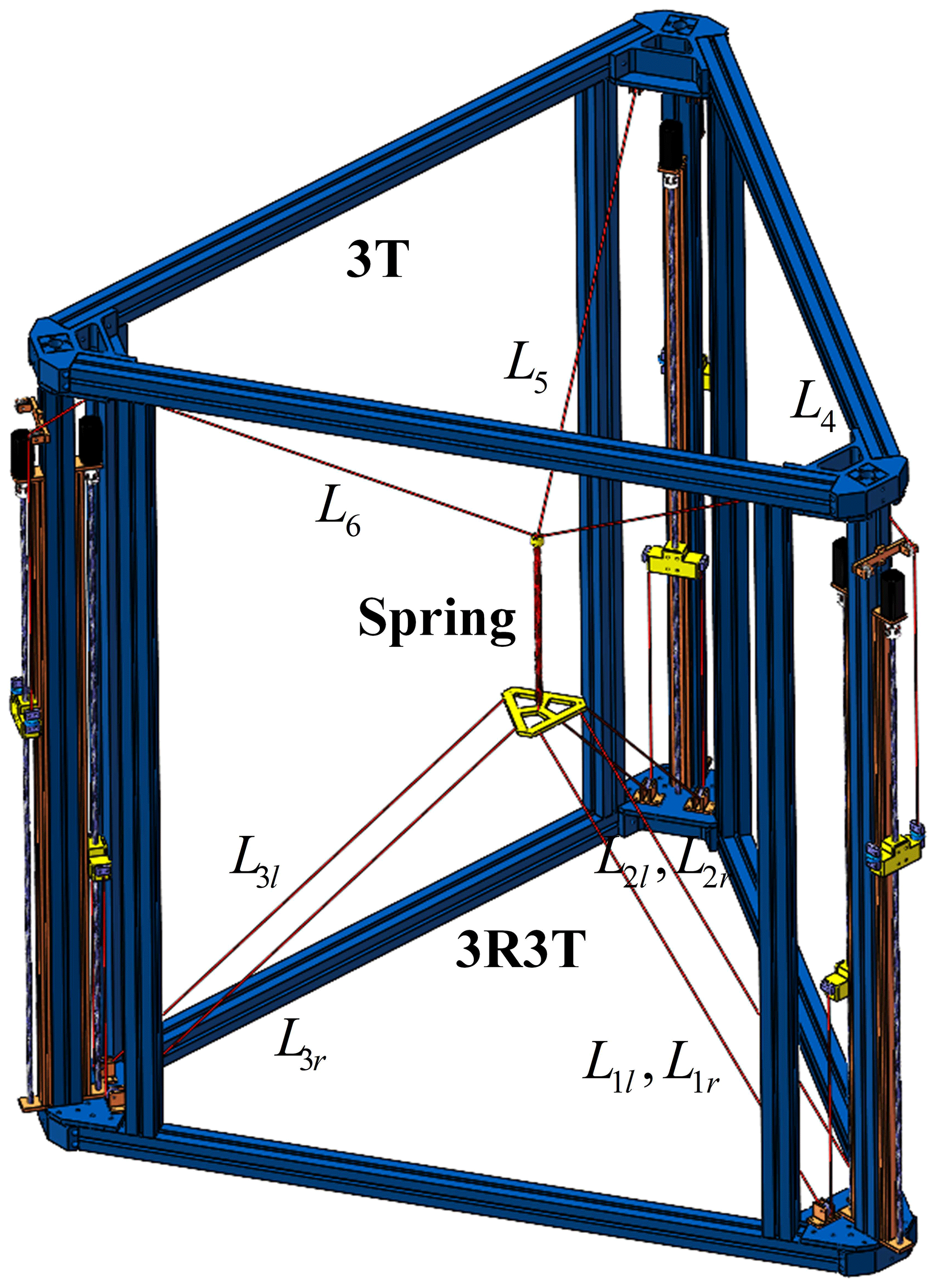
The CDHR mechanism, as illustrated in Fig. 1, is comprised of a 3T parallel mechanism and a 3R3T parallel mechanism connected in series by a spring. The 3T parallel mechanism is made up of three independent cables $L_i(i=\mathrm{4},\mathrm{5},\mathrm{6})$ used for adjusting the spring length. The 3R3T mechanism comprises three parallelogram mechanisms, each consisting of a set of parallel cables L_il, $L_{ir}(i=\mathrm{1},\mathrm{2},\mathrm{3})$, which are utilized to constrain the three rotational DOFs of the end-effector. The spring is utilized to ensure the mechanism's stiffness and to connect the 3T parallel mechanism to the 3R3T parallel mechanism, enabling control and adjustment of the tension in the nine cables.

Figure 1 Mechanism diagram.

2.2 Mechanism equivalence and error analysis

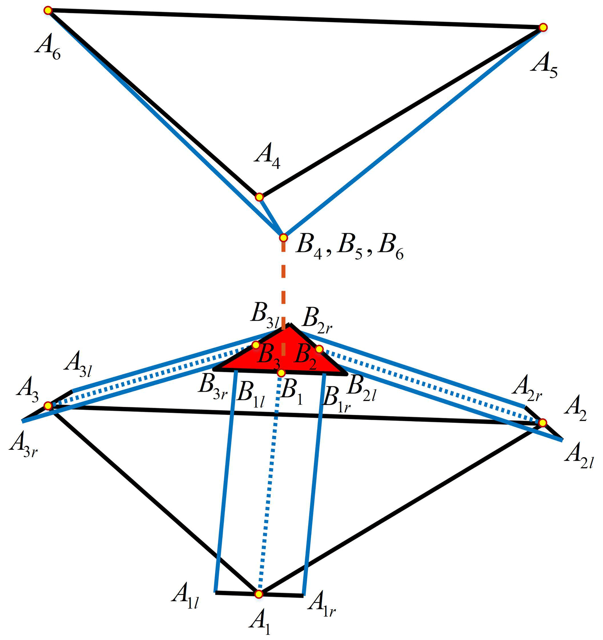
Based on the parallel configuration, the three groups of parallel cables L_il, $L_{ir}(i=\mathrm{1},\mathrm{2},\mathrm{3})$ in the 3R3T mechanism be equivalently simplified as three individual cables $L_i(i=\mathrm{1},\mathrm{2},\mathrm{3})$ for analysis. After the equivalence, the kinematics and dynamics analysis of the mechanism is greatly simplified. The equivalent diagram of the 3R3T mechanism is shown in Fig. 2.

Figure 2 Equivalent diagram.

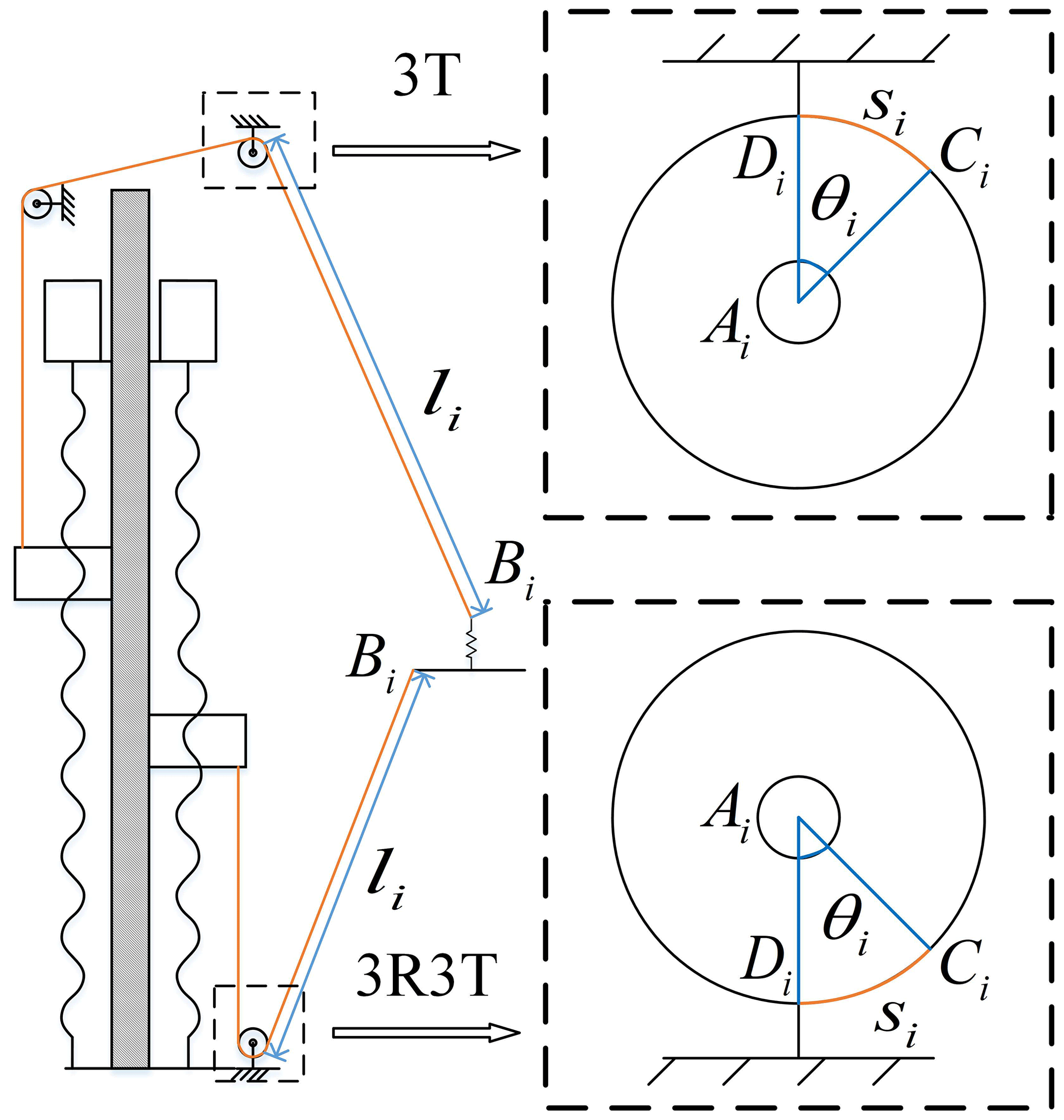
In the cable-driven mechanism, cables are usually guided by multiple pulley systems, and the cable-winding method must be designed accordingly. In this paper, a ball screw slider is used to control the movement of the cables. The cables are connected to the end-effector using the same-side winding method guided by a fixed pulley system. The length of the cable is controlled by the slider's motion to realize the control of the end-effector. In the mechanism analysis, the error generated by the pulley system in the transmission is compensated for, which effectively improves the accuracy of the end-effector's motion. Therefore, the following assumptions are made before the mechanism analysis: no axial sliding of the cable occurs in the groove of the fixed pulley, and there is no cable deformation.

Under the given assumptions, cables are connected to the end-effector, guided by multiple pulley systems. The working diagram is illustrated in Fig. 3. The centre of each pulley is represented by A_i. The global coordinate system O–XYZ is established in the plane where the pulley centres ${\mathit{A}}_i(i=\mathrm{1},\mathrm{2},\mathrm{3})$ are located. The origin of this coordinate system, denoted by O, corresponds to the centre of the triangle formed by the fixed pulley centres A_i. The positive direction of the X axis is defined by the vector OA₁, while the Z axis points vertically upward. The connection point between the cable and the end-effector is denoted by B_i. The direction of the cable from the slider to the fixed pulley is determined during the movement of the end-effector, whereas the direction of the cable from the fixed pulley to the end-effector varies with the motion of the end-effector. Consequently, there exists a moving point C_i and a fixed point D_i on the fixed pulley. C_i represents the dynamic tangent point of the cable and the fixed pulley. D_i is a fixed point that does not affect the length increment of the cable L_i. The length of the arc is denoted as $\stackrel{⌢}{\mathit{C}{\mathit{D}}_i}$, and the corresponding angle is θ_i. During the analysis, the length of the cable l_i is calculated from the point D_i. Then,

$$\begin{array}{}\text{(1)}& l_i=s_i+∥{\mathit{B}}_i{\mathit{C}}_i∥(i=\mathrm{1},\mathrm{2},\mathrm{\dots },\mathrm{6}).\end{array}$$

Figure 3 Working diagram of the pulley system.

2.3 Kinematics analysis

The trajectories of the end-effectors of the 3R3T mechanism and the 3T mechanism are ${\mathit{q}}_{\mathrm{3}r\mathrm{3}t}={\left[\begin{array}{ccc}{x}_{\mathrm{3}r\mathrm{3}t}& y_{\mathrm{3}r\mathrm{3}t}& z_{\mathrm{3}r\mathrm{3}t}\end{array}\right]}^{\mathrm{T}}$ and ${\mathit{q}}_{\mathrm{3}t}={\left[\begin{array}{ccc}{x}_{\mathrm{3}t}& y_{\mathrm{3}t}& z_{\mathrm{3}t}\end{array}\right]}^{\mathrm{T}}$ respectively; thus

$$\begin{array}{}\text{(2)}& {\mathit{B}}_i{\mathit{A}}_i={\mathit{q}}_{i\mathrm{0}}-{\mathit{q}}_i={\left[\begin{array}{ccc}{x}_i& y_i& z_i\end{array}\right]}^{\mathrm{T}}(i=\mathrm{1},\mathrm{2},\mathrm{\dots },\mathrm{6}),\end{array}$$

where q_i0 is the spatial vector B_iA_i at the initial moment, q_i is the motion trajectory of the end-effector, and ${\mathit{q}}_{\mathrm{1}}={\mathit{q}}_{\mathrm{2}}={\mathit{q}}_{\mathrm{3}}={\mathit{q}}_{\mathrm{3}r\mathrm{3}t}$ and ${\mathit{q}}_{\mathrm{4}}={\mathit{q}}_{\mathrm{5}}={\mathit{q}}_{\mathrm{6}}={\mathit{q}}_{\mathrm{3}t}$.

According to the space geometry, the implicit expression of θ_i is as follows:

$$\begin{array}{}\text{(3)}& r+\left|z_i\right|\cos \left({\mathit{\theta }}_i\right)=\left|\sqrt{x_i^{\mathrm{2}}+y_i^{\mathrm{2}}}\right|\sin \left({\mathit{\theta }}_i\right)(i=\mathrm{1},\mathrm{2},\mathrm{\dots },\mathrm{6}),\end{array}$$

where r is the radius of the fixed pulley. Then, according to Eq. (3), θ_i can be expressed as follows:

$$\begin{array}{}\text{(4)}& {\mathit{\theta }}_i=\arcsin \left({\displaystyle \frac{r}{\sqrt{{\left|x_i\right|}^{\mathrm{2}}+{\left|y_i\right|}^{\mathrm{2}}+{\left|z_i\right|}^{\mathrm{2}}}}}\right)+\arctan \left({\displaystyle \frac{\left|z_i\right|}{\sqrt{x_i^{\mathrm{2}}+y_i^{\mathrm{2}}}}}\right).\end{array}$$

The kinematics analysis of the mechanism is the mapping relationship between the cable length $\mathit{l}={\left[\begin{array}{cccccc}{l}_{\mathrm{1}}& l_{\mathrm{2}}& l_{\mathrm{3}}& l_{\mathrm{4}}& l_{\mathrm{5}}& l_{\mathrm{6}}\end{array}\right]}^{\mathrm{T}}$ and the end-effector motion trajectory $\mathit{q}={\left[\begin{array}{cccccc}{x}_{\mathrm{3}r\mathrm{3}t}& y_{\mathrm{3}r\mathrm{3}t}& z_{\mathrm{3}r\mathrm{3}t}& x_{\mathrm{3}t}& y_{\mathrm{3}t}& z_{\mathrm{3}t}\end{array}\right]}^{\mathrm{T}}$. Firstly, according to θ_i, the expression of s_i is

$$\begin{array}{}\text{(5)}& s_i=\stackrel{⌢}{{\mathit{C}}_i{\mathit{D}}_i}=r{\mathit{\theta }}_i.\end{array}$$

According to Eq. (5), it can be obtained such that

$$\begin{array}{}\text{(6)}& \begin{array}{rl}& {\mathit{A}}_i{\mathit{C}}_i\\ & ={\left[\begin{array}{ccc}-r\sin \left({\mathit{\theta }}_i\right)\cos \left({\mathit{\beta }}_i\right)& r\sin \left({\mathit{\theta }}_i\right)\sin \left({\mathit{\beta }}_i\right)& \frac{z_i}{\left|z_i\right|}r\cos \left({\mathit{\beta }}_i\right)\end{array}\right]}^{\mathrm{T}},\end{array}\end{array}$$

where β_i is the angle between the fixed pulley cross section A_iC_iD_i and the coordinate system plane XOZ. Since ${\mathit{B}}_i{\mathit{C}}_i^{\mathrm{T}}{\mathit{A}}_i{\mathit{C}}_i={\mathit{A}}_i{\mathit{C}}_i^{\mathrm{T}}{\mathit{B}}_i{\mathit{C}}_i=\mathrm{0}$, then

$$\begin{array}{}\text{(7)}& \begin{array}{rl}{∥{\mathit{B}}_i{\mathit{A}}_i∥}^{\mathrm{2}}& ={∥{\mathit{B}}_i{\mathit{C}}_i-{\mathit{A}}_i{\mathit{C}}_i∥}^{\mathrm{2}}\\ & ={\mathit{B}}_i{\mathit{C}}_i^{\mathrm{T}}{\mathit{B}}_i{\mathit{C}}_i+{\mathit{A}}_i{\mathit{C}}_i^{\mathrm{T}}{\mathit{A}}_i{\mathit{C}}_i.\end{array}\end{array}$$

According to Eq. (1), for the length of the cable, the system of equations can be obtained as follows:

$$\begin{array}{}\text{(8)}& {\left(l_i-s_i\right)}^{\mathrm{2}}-B_i{A}_i^T{B}_i{A}_i+A_i{C}_i^T{A}_i{C}_i=\mathrm{0}(i=\mathrm{1},\mathrm{2},\mathrm{\dots },\mathrm{6}).\end{array}$$

According to Eqs. (1)–(8), the mapping relationship between end-effector trajectory q and cable length l can be obtained as follows:

$$\begin{array}{}\text{(9)}& \mathit{l}=\mathit{l}\left(\mathit{q}\right)=\mathit{s}+{\mathbf{\Delta }}_L,\end{array}$$

where, $\mathit{s}={\left[\begin{array}{cccccc}{s}_{\mathrm{1}}& s_{\mathrm{2}}& s_{\mathrm{3}}& s_{\mathrm{4}}& s_{\mathrm{5}}& s_{\mathrm{6}}\end{array}\right]}^{\mathrm{T}}$, and ${\mathbf{\Delta }}_L={\left({\mathrm{\Delta }}_{Li}\right)}_{\mathrm{6}\times \mathrm{1}}=\sqrt{{\mathit{B}}_i{\mathit{A}}_i^{\mathrm{T}}{\mathit{B}}_i{\mathit{A}}_i-{\mathit{A}}_i{\mathit{C}}_i^{\mathrm{T}}{\mathit{A}}_i{\mathit{C}}_i}(i=\mathrm{1},\mathrm{2},\mathrm{\dots },\mathrm{6})$.

2.4 Dynamics analysis

The dynamics of the mechanism are analysed by the Newton–Euler method considering the pulley effect. The masses of the end-effectors of 3R3T and 3T are m_3r3t and m_3t, respectively. The vectors of the tensile forces provided by the springs on the 3R3T and 3T mechanisms are F_k3r3t and F_k3t, respectively; thus, the spring tension ${\mathit{F}}_k={\left[\begin{array}{cc}{\mathit{F}}_{k\mathrm{3}r\mathrm{3}t}^{\mathrm{T}}& {\mathit{F}}_{k\mathrm{3}t}^{\mathrm{T}}\end{array}\right]}^{\mathrm{T}}$. The direction ${\mathit{e}}_i={\left[\begin{array}{ccc}{e}_{ix}& e_{iy}& e_{iz}\end{array}\right]}^{\mathrm{T}}$ of the cable force F_i provided by the cable on the end-effector is the directional vector of B_iC_i; thus

$$\begin{array}{}\text{(10)}& {\mathit{e}}_i={\displaystyle \frac{{\mathit{B}}_i{\mathit{C}}_i}{∥{\mathit{B}}_i{\mathit{C}}_i∥}}={\displaystyle \frac{{\mathit{B}}_i{\mathit{A}}_i+{\mathit{A}}_i{\mathit{C}}_i}{l_i-s_i}}(i=\mathrm{1},\mathrm{2},\mathrm{\dots },\mathrm{6}).\end{array}$$

According to Eq. (10), the cable force F_i=f_ie_i is obtained, and f_i is the scalar magnitude of the cable force. Therefore, the kinetic equation of the end-effector is

$$\begin{array}{}\text{(11)}& \mathbf{J}\mathit{F}+{\mathit{F}}_k+\mathit{G}=\mathbf{M}\ddot{\mathit{q}},\end{array}$$

where $\ddot{\mathit{q}}={\left[\begin{array}{cccccc}{\ddot{x}}_{\mathrm{3}r\mathrm{3}t}& {\ddot{y}}_{\mathrm{3}r\mathrm{3}t}& {\ddot{z}}_{\mathrm{3}r\mathrm{3}t}& {\ddot{x}}_{\mathrm{3}t}& {\ddot{y}}_{\mathrm{3}t}& {\ddot{z}}_{\mathrm{3}t}\end{array}\right]}^{\mathrm{T}}$, $\mathbf{G}={\left[\begin{array}{cccccc}\mathrm{0}& \mathrm{0}& -m_{\mathrm{3}r\mathrm{3}t}g& \mathrm{0}& \mathrm{0}& -m_{\mathrm{3}t}g\end{array}\right]}^{\mathrm{T}}$, g is gravitational acceleration, $\mathit{F}={\left[\begin{array}{cccccc}{f}_{\mathrm{1}}& f_{\mathrm{2}}& f_{\mathrm{3}}& f_{\mathrm{4}}& f_{\mathrm{5}}& f_{\mathrm{6}}\end{array}\right]}^{\mathrm{T}}$,

$$\begin{array}{c}{\displaystyle }{\mathbf{J}}_{\mathrm{3}r\mathrm{3}t}={\left[\begin{array}{ccc}{\mathit{e}}_{\mathrm{1}}& {\mathit{e}}_{\mathrm{2}}& {\mathit{e}}_{\mathrm{3}}\end{array}\right]}^{\mathrm{T}},{\mathbf{J}}_{\mathrm{3}t}={\left[\begin{array}{ccc}{\mathit{e}}_{\mathrm{4}}& {\mathit{e}}_{\mathrm{5}}& {\mathit{e}}_{\mathrm{6}}\end{array}\right]}^{\mathrm{T}},\\ {\displaystyle }\mathbf{J}=\left[\begin{array}{cc}{\mathbf{J}}_{\mathrm{3}r\mathrm{3}t}& \mathbf{0}\\ \mathbf{0}& {\mathbf{J}}_{\mathrm{3}t}\end{array}\right],{\mathbf{M}}_{\mathrm{3}r\mathrm{3}t}=\left[\begin{array}{ccc}{m}_{\mathrm{3}r\mathrm{3}t}& \mathrm{0}& \mathrm{0}\\ \mathrm{0}& m_{\mathrm{3}r\mathrm{3}t}& \mathrm{0}\\ \mathrm{0}& \mathrm{0}& m_{\mathrm{3}r\mathrm{3}t}\end{array}\right],\\ {\displaystyle }{\mathbf{M}}_{\mathrm{3}t}=\left[\begin{array}{ccc}{m}_{\mathrm{3}t}& \mathrm{0}& \mathrm{0}\\ \mathrm{0}& m_{\mathrm{3}t}& \mathrm{0}\\ \mathrm{0}& \mathrm{0}& m_{\mathrm{3}t}\end{array}\right],\mathbf{M}=\left[\begin{array}{cc}{\mathbf{M}}_{\mathrm{3}r\mathrm{3}t}& \mathbf{0}\\ \mathbf{0}& {\mathbf{M}}_{\mathrm{3}t}\end{array}\right],\\ {\displaystyle }{F}_{k\mathrm{3}r\mathrm{3}t}=k\left({\mathit{B}}_{\mathrm{4}}-{\displaystyle \frac{\mathrm{1}}{\mathrm{3}}}({\mathit{B}}_{\mathrm{1}}+{\mathit{B}}_{\mathrm{2}}+{\mathit{B}}_{\mathrm{3}})\right),\end{array}$$

and $F_{k\mathrm{3}t}=k\left(\frac{\mathrm{1}}{\mathrm{3}}({\mathit{B}}_{\mathrm{1}}+{\mathit{B}}_{\mathrm{2}}+{\mathit{B}}_{\mathrm{3}})-{\mathit{B}}_{\mathrm{4}}\right)$, where k is spring stiffness.

According to Eq. (11), the expression of the cable force F is

$$\begin{array}{}\text{(12)}& \mathit{F}\left(\mathit{q},\dot{\mathit{q}},\ddot{\mathit{q}}\right)={\mathbf{J}}^{-\mathrm{1}}\left(\mathbf{M}\ddot{\mathit{q}}-{\mathit{F}}_k-\mathit{G}\right).\end{array}$$

2.5 Cable forces analysis

The cable forces $f_i(i=\mathrm{1},\mathrm{2},\mathrm{3})$ of the 3R3T mechanism obtained from Eq. (12) are provided by three groups of parallel cables. It is known that the cable forces f_ir=e_if_ir and ${\mathit{f}}_{il}={\mathit{e}}_i{\mathit{f}}_{il}(i=\mathrm{1},\mathrm{2},\mathrm{3})$ provide the actual cable force values by distributing the equivalent cable forces (${\mathit{f}}_i(i=\mathrm{1},\mathrm{2},\mathrm{3})$). Therefore, the cable forces satisfy the torque balance condition as follows:

$$\begin{array}{}\text{(13)}& \begin{array}{ll}\left\{\begin{array}{l}\sum _{i=\mathrm{1}}^{\mathrm{3}}\left({\mathit{r}}_{ir}\times {\mathit{f}}_{ir}+{\mathit{r}}_{il}\times {\mathit{f}}_{il}\right)=\mathbf{0}\\ f_i=f_{ir}+f_{il}\end{array}\right.& (i=\mathrm{1},\mathrm{2},\mathrm{3}),\end{array}\end{array}$$

where ${\mathit{r}}_{ir}={\left[\begin{array}{ccc}{r}_{irx}& r_{iry}& r_{irz}\end{array}\right]}^{\mathrm{T}}$ and ${\mathit{r}}_{il}={\left[\begin{array}{ccc}{r}_{ilx}& r_{ily}& r_{ilz}\end{array}\right]}^{\mathrm{T}}$ are constants determined by the size of the end-effector. According to Eq. (13), cable forces ${\mathit{f}}_r={\left[\begin{array}{ccc}{f}_{\mathrm{1}r}& f_{\mathrm{2}r}& f_{\mathrm{3}r}\end{array}\right]}^{\mathrm{T}}$, ${\mathit{f}}_l={\left[\begin{array}{ccc}{f}_{\mathrm{1}l}& f_{\mathrm{2}l}& f_{\mathrm{3}l}\end{array}\right]}^{\mathrm{T}}$, and $\mathit{f}={\left[\begin{array}{ccc}{f}_{\mathrm{1}}& f_{\mathrm{2}}& f_{\mathrm{3}}\end{array}\right]}^{\mathrm{T}}$ can be calculated as follows:

$$\begin{array}{}\text{(14)}& \left\{\begin{array}{l}{\mathit{f}}_r=-{\mathbf{D}}^{-\mathrm{1}}{\mathbf{D}}_l\mathit{f}\\ {\mathit{f}}_l={\mathbf{D}}^{-\mathrm{1}}{\mathbf{D}}_r\mathit{f}\end{array},\right.\end{array}$$

where ${\mathit{r}}_i={\mathit{r}}_{ir}-{\mathit{r}}_{il}={\left[\begin{array}{ccc}{r}_{ix}& r_{iy}& r_{iz}\end{array}\right]}^{\mathrm{T}}$,
$\mathbf{D}=\left[\begin{array}{ccc}{\mathit{r}}_{\mathrm{1}}\times {\mathit{e}}_{\mathrm{1}}& {\mathit{r}}_{\mathrm{2}}\times {\mathit{e}}_{\mathrm{2}}& {\mathit{r}}_{\mathrm{3}}\times {\mathit{e}}_{\mathrm{3}}\end{array}\right]$,
${\mathbf{D}}_l=\left[\begin{array}{ccc}{\mathit{r}}_{\mathrm{1}l}\times {\mathit{e}}_{\mathrm{1}}& {\mathit{r}}_{\mathrm{2}l}\times {\mathit{e}}_{\mathrm{2}}& {\mathit{r}}_{\mathrm{3}l}\times {\mathit{e}}_{\mathrm{3}}\end{array}\right]$, and
${\mathbf{D}}_r=\left[\begin{array}{ccc}{\mathit{r}}_{\mathrm{1}r}\times {\mathit{e}}_{\mathrm{1}}& {\mathit{r}}_{\mathrm{2}r}\times {\mathit{e}}_{\mathrm{2}}& {\mathit{r}}_{\mathrm{3}r}\times {\mathit{e}}_{\mathrm{3}}\end{array}\right]$.

3 Simulation design and analysis verification

3.1 Simulation design

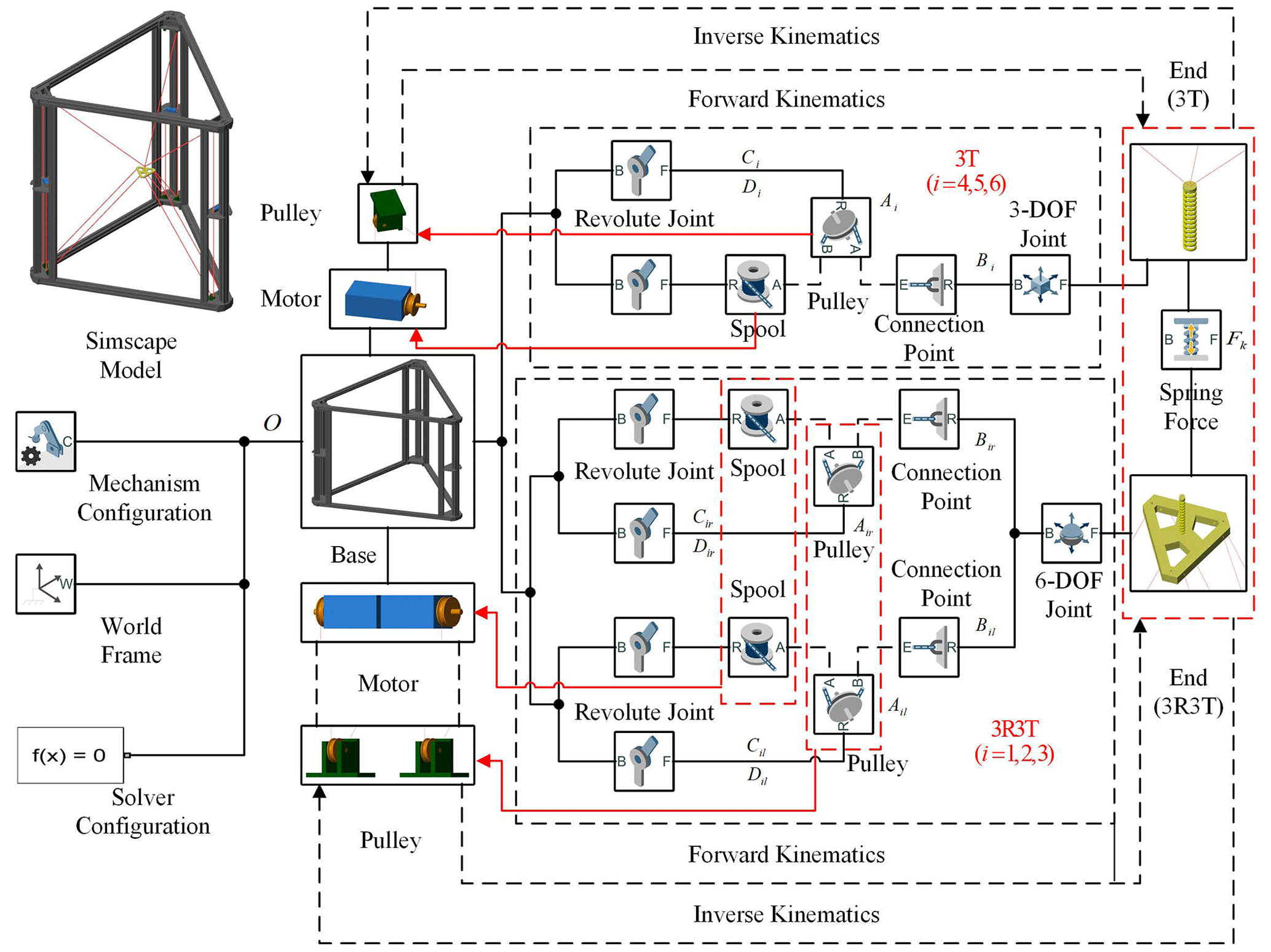
Here, we compare the simulation software of ADAMS and Simscape for the cable-driven mechanism. ADAMS can build the simulation environment by setting the parameters of anchor, puller, and cable in the cable module, which can realize the simulation of the tensile deformation of the cable. However, solving the parameters and implementing the controller in the simulation is challenging. Therefore, the simulation analysis of the cable-driven mechanism is usually realized by using an ADAMS–Simulink joint simulation. Simscape can build the simulation environment by configuring the parameters of belt-cable end, belt-cable spool, belt-cable properties, and pulley in the belts and cables modules. The simulation process does not take into account the cable deformation, but it can enable complex trajectory planning and controller simulation. Additionally, utilizing Simulink's visual interface can realize the digital twin of the experimental process and realize the interaction between the simulation and the actual working conditions. To validate the analysis of this mechanism in Sect. 2, the motor-driven cable spool is utilized, and the cable is connected to the end-effector through the guidance of a pulley system. Figure 4 displays the simulation environment of the mechanism built with Simscape. In the kinematic and dynamical analysis of the mechanism, the specific parameters are shown in Appendix A. The two end-effectors are verified with the same trajectory, the following specific trajectory expression:

$$\begin{array}{}\text{(15)}& \left\{\begin{array}{l}x={\ln }^{\mathrm{3}}(\mathrm{0.5}t+\mathrm{1})\cos \left(\mathrm{0.03}\mathit{\pi }t\right)\\ y={\ln }^{\mathrm{3}}(\mathrm{0.5}t+\mathrm{1})\sin \left(\mathrm{0.03}\mathit{\pi }t\right)\\ z={\ln }^{\mathrm{3}}(t+\mathrm{1})\end{array},\right.(\mathrm{0}\le t<\mathrm{200})\end{array}$$

where x, y, and z are the displacements of the end-effector in X, Y, and Z directions in millimetres (mm), and t is the simulation time in seconds (s).

Figure 4 Simscape mechanism model.

In order to analyse the motion of the mechanism in space, the cable is driven by the belt–cable spool in the simulation. Apart from obtaining the cable force as described in Eqs. (10)–(14), the belt-cable spool also needs to satisfy the required acceleration ${\ddot{l}}_i$ of the cable during dynamic simulation. Thus, the dynamic equation relating the cable force to the torque exerted on the belt-cable spool is established as follows:

$$\begin{array}{}\text{(16)}& \begin{array}{ll}\left\{\begin{array}{l}{f}_{i}r+t_i=I_i{\mathit{\alpha }}_i\\ {\mathit{\alpha }}_i=\frac{{\ddot{l}}_i}{r}\end{array}\right.& (i=\mathrm{1},\mathrm{2},\mathrm{\dots },\mathrm{6})\end{array},\end{array}$$

where t_i is the torque provided by the belt-cable spool, I_i is the rotational inertia of the belt-cable spool, and α_i is the angular acceleration of the belt-cable spool. To simplify the calculation, the fixed-pulley section S_ΔAOD is rotated to the coordinate system plane S_XOZ for normalization; following this, the vector B_iA_i normalized to the vector BA_i satisfies

$$\begin{array}{}\text{(17)}& {\mathit{B}}_i{\mathit{A}}_i={\mathbf{R}}_{zi}\mathit{B}{\mathit{A}}_i={\left[\begin{array}{ccc}{x}_{in}& y_{in}& z_{in}\end{array}\right]}^{\mathrm{T}}(i=\mathrm{1},\mathrm{2},\mathrm{\dots },\mathrm{6}),\end{array}$$

where

$${\mathbf{R}}_{zi}={\mathbf{R}}_z\left({\mathit{\beta }}_i\right)=\left[\begin{array}{ccc}\cos {\mathit{\beta }}_i& -\sin {\mathit{\beta }}_i& \mathrm{0}\\ \sin {\mathit{\beta }}_i& \cos {\mathit{\beta }}_i& \mathrm{0}\\ \mathrm{0}& \mathrm{0}& \mathrm{1}\end{array}\right].$$

According to Eq. (17), Eq. (3) can be simplified as follows:

$$\begin{array}{}\text{(18)}& r+\left|z_{in}\right|\cos \left({\mathit{\theta }}_i\right)=\left|x_{in}\right|\sin \left({\mathit{\theta }}_i\right)(i=\mathrm{1},\mathrm{2},\mathrm{\dots },\mathrm{6}).\end{array}$$

The implicit expressions for ${\dot{\mathit{\theta }}}_i$ and ${\ddot{\mathit{\theta }}}_i$ are obtained by simultaneously taking the first- and second-order derivatives for time t on both sides:

$$\begin{array}{}\text{(19)}& \left\{\begin{array}{l}{k}_i\left({\dot{z}}_{in}-z_{in}\tan \left({\mathit{\theta }}_i\right){\dot{\mathit{\theta }}}_i\right)={\dot{x}}_{in}\tan \left({\mathit{\theta }}_i\right)+x_{in}{\dot{\mathit{\theta }}}_i\\ k_i\left({\ddot{z}}_{in}-\mathrm{2}{\dot{z}}_{in}\tan \left({\mathit{\theta }}_i\right){\dot{\mathit{\theta }}}_i-z_{in}{\dot{\mathit{\theta }}}_i^{\mathrm{2}}-z_{in}\tan \left({\mathit{\theta }}_i\right){\ddot{\mathit{\theta }}}_i\right)\\ ={\ddot{x}}_{in}\tan \left({\mathit{\theta }}_i\right)+\mathrm{2}{\dot{x}}_{in}{\dot{\mathit{\theta }}}_i-x_{in}\tan \left({\mathit{\theta }}_i\right){\dot{\mathit{\theta }}}_i^{\mathrm{2}}+x_{in}{\ddot{\mathit{\theta }}}_i\end{array},\right.\end{array}$$

where $k_i=\frac{z_{in}}{\left|z_{in}\right|}$, and the expressions for ${\dot{\mathit{\theta }}}_i$ and ${\ddot{\mathit{\theta }}}_i$ are as follows:

$$\begin{array}{}\text{(20)}& \left\{\begin{array}{l}{\dot{\mathit{\theta }}}_i=\frac{k_i{\dot{z}}_{in}-{\dot{x}}_{in}\tan \left({\mathit{\theta }}_i\right)}{k_i{z}_{in}\tan \left({\mathit{\theta }}_i\right)+x_{in}}\\ \begin{array}{rl}{\ddot{\mathit{\theta }}}_i& =\left(x_{in}\tan \left({\mathit{\theta }}_i\right)-k_i{\dot{z}}_{in}\right){\dot{\mathit{\theta }}}_i^{\mathrm{2}}-\mathrm{2}({\dot{x}}_{in}+k_i{\dot{z}}_{in}\tan ({\mathit{\theta }}_i\left)\right){\dot{\mathit{\theta }}}_i\\ & +\left(k_i{\ddot{z}}_{in}-{\ddot{x}}_{in}\tan \left({\mathit{\theta }}_i\right)\right)\backslash \left(x_{in}+k_i{z}_{in}\tan \left({\mathit{\theta }}_i\right)\right)\end{array}\end{array}.\right.\end{array}$$

Taking the first- and second-order derivatives of both sides of Eq. (7) simultaneously for time t, we obtain ${\dot{l}}_i$ and ${\ddot{l}}_i$ as follows:

$$\begin{array}{}\text{(21)}& \left\{\begin{array}{l}{\dot{l}}_i={\dot{s}}_i+\frac{{\mathit{B}}_i{\mathit{C}}_i^{\mathrm{T}}\dot{{\mathit{B}}_i{\mathit{C}}_i}}{l_i-s_i}\\ {\ddot{l}}_i={\ddot{s}}_i+{\displaystyle \frac{{\mathit{B}}_i{\mathit{C}}_i^{\mathrm{T}}\ddot{{\mathit{B}}_i{\mathit{C}}_i}+{\dot{{\mathit{B}}_i{\mathit{C}}_i}}^{\mathrm{T}}\dot{{\mathit{B}}_i{\mathit{C}}_i}-({\dot{l}}_i-{\dot{s}}_i{)}^{\mathrm{2}}}{l_i-s_i}}\end{array},\right.\end{array}$$

where ${\dot{s}}_i=r{\dot{\mathit{\theta }}}_i$, ${\ddot{s}}_i=r{\ddot{\mathit{\theta }}}_i$,

$${\displaystyle }\dot{{\mathit{B}}_i{\mathit{C}}_i}=\left[\begin{array}{c}{\dot{x}}_i-r\cos \left({\mathit{\beta }}_i\right)\cos \left({\mathit{\theta }}_i\right){\dot{\mathit{\theta }}}_i\\ {\dot{y}}_i+r\sin \left({\mathit{\beta }}_i\right)\cos \left({\mathit{\theta }}_i\right){\dot{\mathit{\theta }}}_i\\ {\dot{z}}_i-\frac{z_i}{\left|z_i\right|}r\sin \left({\mathit{\theta }}_i\right){\dot{\mathit{\theta }}}_i\end{array}\right],$$

and

$${\displaystyle }\ddot{{\mathit{B}}_i{\mathit{C}}_i}=\left[\begin{array}{c}{\ddot{x}}_i+r\cos \left({\mathit{\beta }}_i\right)\left(\sin \left({\mathit{\theta }}_i\right){\dot{\mathit{\theta }}}_i^{\mathrm{2}}-\cos \left({\mathit{\theta }}_i\right){\ddot{\mathit{\theta }}}_i\right)\\ {\ddot{y}}_i-r\sin \left({\mathit{\beta }}_i\right)\left(\sin \left({\mathit{\theta }}_i\right){\dot{\mathit{\theta }}}_i^{\mathrm{2}}+\cos \left({\mathit{\theta }}_i\right){\ddot{\mathit{\theta }}}_i\right)\\ {\ddot{z}}_i-\frac{z_i}{\left|z_i\right|}r\left(\cos \left({\mathit{\theta }}_i\right){\dot{\mathit{\theta }}}_i^{\mathrm{2}}-\sin \left({\mathit{\theta }}_i\right){\ddot{\mathit{\theta }}}_i\right)\end{array}\right].$$

According to the kinematics and dynamics derivation, the required torque of the belt-cable spool can be obtained by bringing Eqs. (17)–(21) into Eq. (16).

3.2 Kinematics simulation

The simulation is conducted based on the kinematics l=l(q) obtained from Eqs. (1)–(9). The objective is to validate the accuracy of the kinematics analysis considering error compensation. A comparison is made between the cable length without error compensation, denoted as l_i=∥B_iA_i∥, and the cable length with error compensation, given by $l_i=s_i+∥{\mathit{B}}_i{\mathit{C}}_i∥$. Furthermore, the end-effector motion error is evaluated based on the results of kinematics simulation. Figure 5a illustrates the end-effector trajectory for the 3R3T mechanism obtained from kinematics simulation. Figure 5b displays the end-effector errors for the 3R3T mechanism in terms of kinematics. Lastly, Fig. 5c provides a comparison of the spring tension.

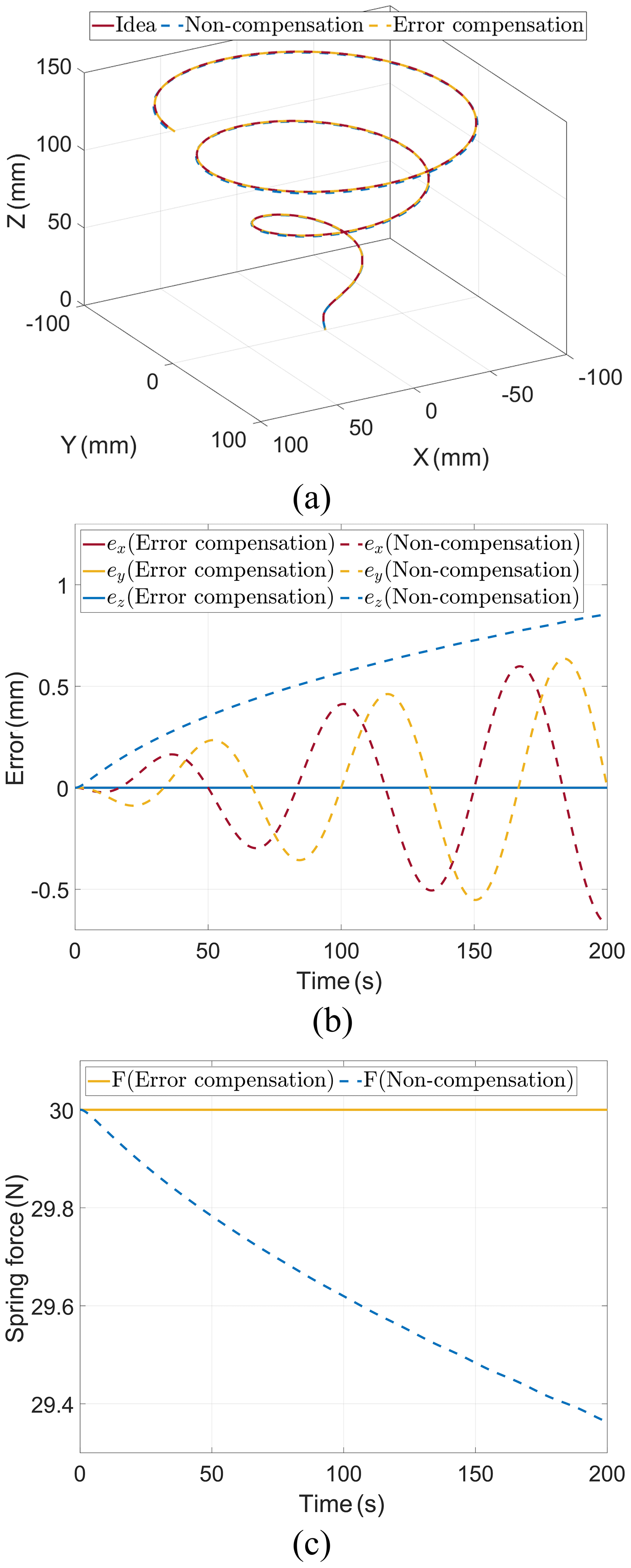
Figure 5 Kinematics simulation. (a) Trajectories of end-effector. (b) Errors of end-effector. (c) Spring tensions.

When error compensation is applied for analysis, the end-effector trajectory matches the kinematics result exactly, and the spring tension remains constant at 30 N. Without error compensation, the 3R3T end-effector trajectory exhibits fluctuation in the X- and Y-axis directions. The maximum X-axis error ${∥{\mathit{e}}_x∥}_{\mathrm{\infty }}=\mathrm{0.669}$ mm, and the maximum Y-axis error ${∥{\mathit{e}}_y∥}_{\mathrm{\infty }}=\mathrm{0.636}$ mm. The error of the 3R3T end-effector gradually increases in the Z-axis direction, with the maximum Z-axis error ${∥{\mathit{e}}_z∥}_{\mathrm{\infty }}=\mathrm{0.855}$ mm. As the end-effector moves, the spring tension exhibits periodic variations in the X- and Y-axis directions while gradually decreasing in the Z-axis direction. In summary, incorporating the effect of pulley radius error in kinematics analysis effectively reduces the overall kinematics error.

3.3 Dynamics simulation

Based on the kinematic analysis considering error compensation and non-compensation, the simulation is conducted using the dynamics $\mathit{F}=\mathit{F}(\mathit{q},\dot{\mathit{q}},\ddot{\mathit{q}})$ derived from Eqs. (10)–(12) and (16)–(21). Figure 6a displays the 3R3T end-effector motion trajectory. Figure 6b illustrates the error in the 3R3T end-effector trajectory. Lastly, Fig. 6c depicts the variation in the spring tension.

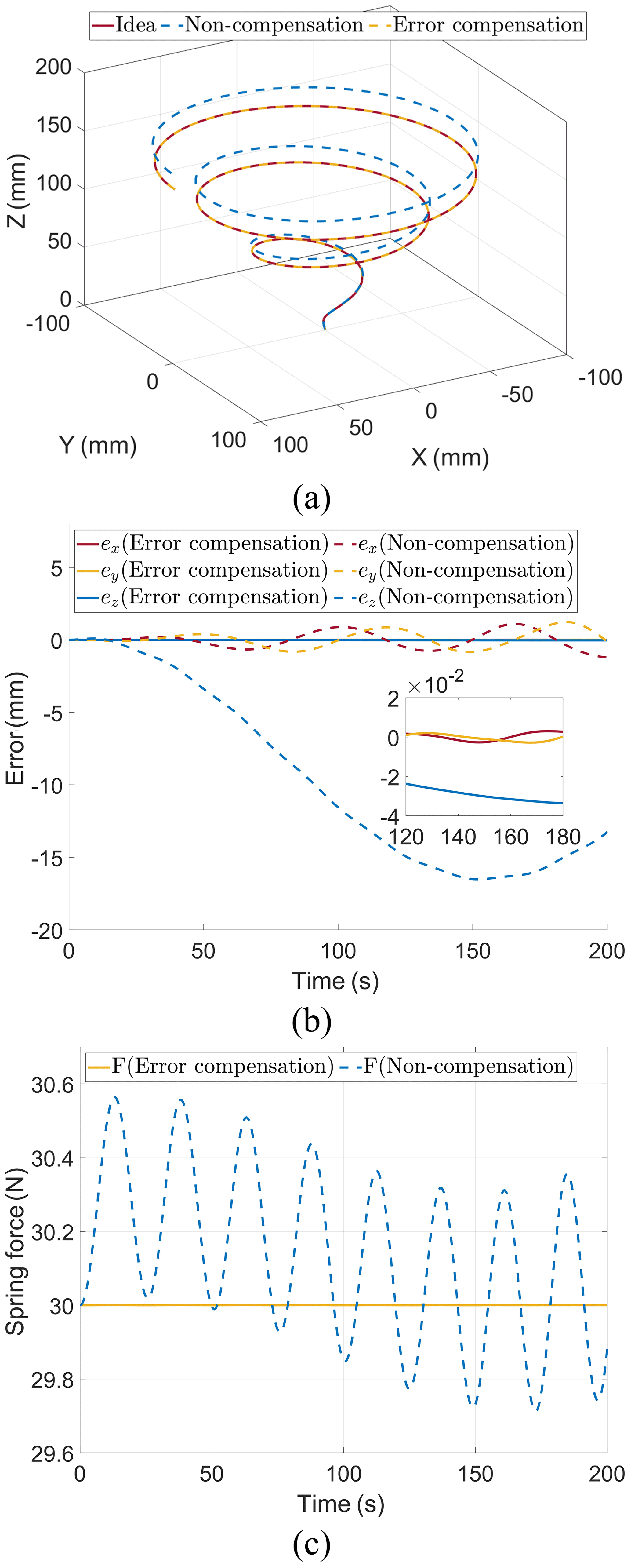
Figure 6 Dynamics simulation. (a) Trajectories of end-effector. (b) Errors of end-effector. (c) Spring tensions.

When there is non-compensation, the maximum X-axis error ${∥{\mathit{e}}_x∥}_{\mathrm{\infty }}=\mathrm{1.213}$ mm, the maximum Y-axis error ${∥{\mathit{e}}_y∥}_{\mathrm{\infty }}=\mathrm{1.228}$ mm, and the maximum Z-axis error ${∥{\mathit{e}}_z∥}_{\mathrm{\infty }}=\mathrm{16.514}$ mm at the end-effector of the 3R3T mechanism. However, after error compensation, the maximum X-axis error is reduced to ${∥{\mathit{e}}_x∥}_{\mathrm{\infty }}=\mathrm{0.003}$ mm, the maximum Y-axis error is reduced to ${∥{\mathit{e}}_y∥}_{\mathrm{\infty }}=\mathrm{0.005}$ mm, and the maximum Z-axis error is reduced to ${∥{\mathit{e}}_z∥}_{\mathrm{\infty }}=\mathrm{0.035}$ mm at the end-effector of 3R3T in the dynamics simulation of the 3R3T mechanism. Furthermore, the spring tension exhibits significant fluctuations following the motion of the end-effector.

Since there is no cumulative error in the kinematics analysis, the error of the end-effector at time t without error compensation is only related to the motion trajectory q and the pulley radius r. However, in the dynamics simulation, the motion error of the end-effector accumulates gradually due to the integration of the cable force F over time t. As a result, the motion error in the dynamics simulation is considerably greater than that in the kinematics simulation. In conclusion, error compensation minimizes the impact of accumulated errors on the end-effector motion and greatly enhances the accuracy of the dynamics simulation.

3.4 Cable force analysis simulation

Based on the kinematic and kinetic analyses, the cable force analysis is conducted based on the distributed cable force f_r and f_l obtained from Eqs.(12)–(13). A comparison is made between the cable force ${\mathit{f}}_r={\mathit{f}}_l=\frac{\mathrm{1}}{\mathrm{2}}{\left[\begin{array}{ccc}{f}_{\mathrm{1}}& f_{\mathrm{2}}& f_{\mathrm{3}}\end{array}\right]}^{\mathrm{T}}$ when not distributed and the effect of the distributed cable force on the motion error of the 3R3T end-effector. Figure  7a displays the end-effector trajectory of the 3R3T mechanism with and without cable force distribution.

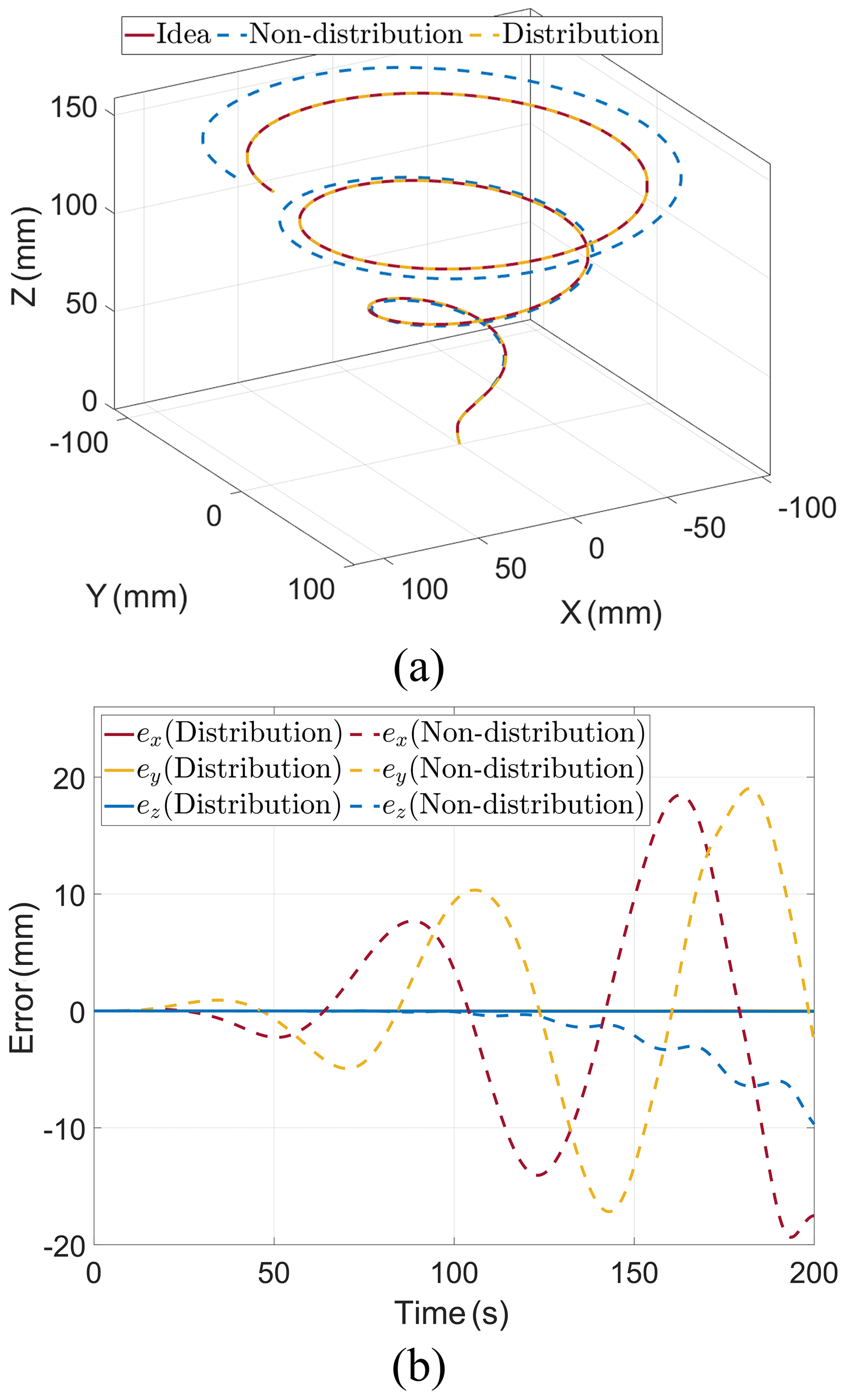
Figure 7 Cable force analysis simulation. (a) Trajectories of end-effector. (b) Errors of end-effector.

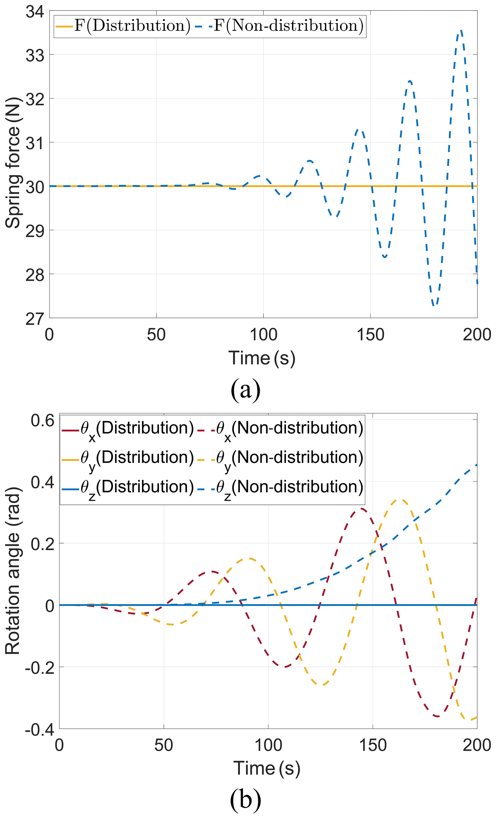
As shown in Fig. 7b, the maximum X-axis error ${∥{\mathit{e}}_x∥}_{\mathrm{\infty }}=\mathrm{19.361}$ mm, the maximum Y-axis error ${∥{\mathit{e}}_y∥}_{\mathrm{\infty }}=\mathrm{19.041}$ mm, and the maximum Z-axis error ${∥{\mathit{e}}_z∥}_{\mathrm{\infty }}=\mathrm{9.682}$ mm when there is no cable force distribution, and the maximum X-axis error ${∥{\mathit{e}}_x∥}_{\mathrm{\infty }}=\mathrm{0.010}$ mm, the maximum Y-axis error ${∥{\mathit{e}}_y∥}_{\mathrm{\infty }}=\mathrm{0.012}$ mm, and the maximum Z-axis error ${∥{\mathit{e}}_z∥}_{\mathrm{\infty }}=\mathrm{0.035}$ mm after cable force distribution. Figure 8a shows the magnitude of the spring force with and without the distribution of the cable force. As shown in Fig. 8b, the maximum X-axis rotation angle ${∥{\mathit{\theta }}_x∥}_{\mathrm{\infty }}=\mathrm{0.360}$ rad, the maximum Y-axis rotation angle ${∥{\mathit{\theta }}_y∥}_{\mathrm{\infty }}=\mathrm{0.373}$ rad, and the maximum Z-axis rotation angle ${∥{\mathit{\theta }}_z∥}_{\mathrm{\infty }}=\mathrm{0.455}$ rad at the end-effector of the 3R3T mechanism without cable force distribution, and the rotation angle θ_x, θ_y, and θ_z≪0.001 rad for the X, Y, and Z axes after the distribution of the cable force. In conclusion, the cable force distribution can significantly improve the accuracy of dynamics analysis and end-effector motion.

Figure 8 Cable force analysis simulation results. (a) Spring tensions. (b) Rotation angle.

4 Controller design and simulation

4.1 Prescribed-performance controller for MIMO (multi-input, multi-output) nonlinear systems

The cable-driven mechanism imposes strict requirements on the cable force range. Consequently, a prescribed-performance controller for cable force is designed. This controller serves the purpose of preventing system performance degradation and ensuring the stability of the closed-loop system. Considering the material properties of the cable, each cable force is restricted within the range of $[f_{imin},f_{imax}]$. According to the system characteristics, the controlled objects are as follows:

$$\begin{array}{}\text{(22)}& \ddot{\mathit{q}}={\mathbf{M}}^{-\mathrm{1}}\left(\mathbf{J}\text{sat}\left(\mathit{F}\right)+{\mathit{F}}_k+\mathbf{G}\right),\end{array}$$

where the input saturation function F_u=sat(F_v) is expressed as follows:

$$\begin{array}{}\text{(23)}& {\mathit{F}}_u=\text{sat}\left({\mathit{F}}_v\right)=\left\{\begin{array}{lr}{f}_{imax},& f_i>f_{imax}\\ f_i,& f_{imin}\le f_i\le f_{imax}\\ f_{imin},& f_i<f_{imin}\end{array}.\right.\end{array}$$

In additive manufacturing, achieving Z-axis accuracy is crucial for fused deposition modelling (FDM). However, the controller alone cannot guarantee that the Z-axis displacement remains within the specified error range at all times, even when the cable satisfies the input saturation function (Eq. 23). As a result, it is necessary to optimize the constrained force. Let F_o represent the actual input that ensures the desired Z-axis displacement error. Consequently, the problem can be formulated as follows:

$$\begin{array}{}\text{(24)}& \left\{\begin{array}{l}{\mathbf{J}}_u{\mathit{F}}_u+{\mathit{F}}_{ku}+\mathit{G}=\mathbf{M}{\ddot{\mathit{q}}}_u\\ {\mathbf{J}}_o{\mathit{F}}_o+{\mathit{F}}_{ko}+\mathit{G}=\mathbf{M}{\ddot{\mathit{q}}}_o.\end{array}\right.\end{array}$$

Taking ε_3r3t and ε_3t to be sufficiently small such that ${\ddot{\mathit{q}}}_o-{\ddot{\mathit{q}}}_u={\left[\begin{array}{cccccc}\mathrm{0}& \mathrm{0}& {\mathit{\epsilon }}_{\mathrm{3}r\mathrm{3}t}& \mathrm{0}& \mathrm{0}& {\mathit{\epsilon }}_{\mathrm{3}t}\end{array}\right]}^{\mathrm{T}}$, the optimized input F_o is obtained as follows:

$$\begin{array}{}\text{(25)}& {\mathit{F}}_o={\mathbf{J}}_o^{-\mathrm{1}}\left({\mathbf{J}}_u{\mathit{F}}_u+{\mathit{F}}_{ku}-{\mathit{F}}_{ko}+\mathbf{M}\left({\ddot{\mathit{q}}}_o\right)-{\ddot{\mathit{q}}}_u\right).\end{array}$$

Then, the auxiliary system is designed:

$$\begin{array}{}\text{(26)}& \dot{\mathit{\lambda }}=\mathbf{A}\mathit{\lambda }+\mathbf{B}\mathrm{\Delta }\mathit{F},\end{array}$$

where

$$\begin{array}{c}{\displaystyle }\mathit{\lambda }={\left[\begin{array}{ccccccc}{\mathit{\lambda }}_{\mathrm{11}}& {\mathit{\lambda }}_{\mathrm{12}}& {\mathit{\lambda }}_{\mathrm{21}}& {\mathit{\lambda }}_{\mathrm{22}}& \mathrm{\cdots }& {\mathit{\lambda }}_{\mathrm{61}}& {\mathit{\lambda }}_{\mathrm{62}}\end{array}\right]}^{\mathrm{T}},\\ {\displaystyle }\mathrm{\Delta }\mathit{F}={\mathit{F}}_o-{\mathit{F}}_v,{\mathbf{A}}_i=\left[\begin{array}{cc}-c_{i\mathrm{1}}& \mathrm{1}\\ \mathrm{0}& -c_{i\mathrm{2}}\end{array}\right],\\ {\displaystyle }\mathbf{A}=\text{diag}({\mathbf{A}}_{\mathrm{1}},{\mathbf{A}}_{\mathrm{2}},\mathrm{\dots },{\mathbf{A}}_{\mathrm{6}}),\end{array}$$

and

$${\displaystyle }\mathbf{B}={\left[\begin{array}{cccccc}\mathrm{0}& b_{\mathrm{1}}& & & & \\ & & \mathrm{0}& b_{\mathrm{2}}& & & \\ & & & & \mathrm{\ddots }& & \\ & & & & & \mathrm{0}& b_{\mathrm{6}}\end{array}\right]}^{\mathrm{T}}.$$

Since A is Hurwitz, i.e. c_i1, c_i2>0. When t→∞, λ_i→0. Meanwhile, to avoid the system instability caused by too-large ΔF, it is necessary to ensure that c_i1 and c_i2 are large enough. The control objective is q_o→q_d, and q_d is the idea motion trajectory of the end-effector. We define the position error as follows:

$$\begin{array}{}\text{(27)}& \mathit{e}={\mathit{q}}_o-{\mathit{q}}_d-{\mathit{\lambda }}_{e\mathrm{1}},\end{array}$$

where ${\mathit{q}}_o={\left[\begin{array}{cccccc}{x}_{o\mathrm{3}r\mathrm{3}t}& y_{o\mathrm{3}r\mathrm{3}t}& z_{o\mathrm{3}r\mathrm{3}t}& x_{o\mathrm{3}t}& y_{o\mathrm{3}t}& z_{o\mathrm{3}t}\end{array}\right]}^{\mathrm{T}}$,
${\mathit{q}}_d={\left[\begin{array}{cccccc}{x}_{d\mathrm{3}r\mathrm{3}t}& y_{d\mathrm{3}r\mathrm{3}t}& z_{d\mathrm{3}r\mathrm{3}t}& x_{d\mathrm{3}t}& y_{d\mathrm{3}t}& z_{d\mathrm{3}t}\end{array}\right]}^{\mathrm{T}}$, and
${\mathit{\lambda }}_{e\mathrm{1}}={\left[\begin{array}{cccc}{\mathit{\lambda }}_{\mathrm{11}}& {\mathit{\lambda }}_{\mathrm{21}}& \mathrm{\cdots }& {\mathit{\lambda }}_{\mathrm{61}}\end{array}\right]}^{\mathrm{T}}$.

Both sides of Eq. (27) are simultaneously derivative with respect to time t:

$$\begin{array}{}\text{(28)}& \dot{\mathit{e}}={\dot{\mathit{q}}}_o-{\dot{\mathit{q}}}_d-{\dot{\mathit{\lambda }}}_{e\mathrm{1}}={\dot{\mathit{q}}}_r-{\dot{\mathit{q}}}_d-{\mathit{\lambda }}_{e\mathrm{2}}+{\mathbf{c}}_{e\mathrm{1}}{\mathit{\lambda }}_{e\mathrm{1}},\end{array}$$

where ${\mathit{\lambda }}_{e\mathrm{2}}={\left[\begin{array}{cccc}{\mathit{\lambda }}_{\mathrm{12}}& {\mathit{\lambda }}_{\mathrm{22}}& \mathrm{\cdots }& {\mathit{\lambda }}_{\mathrm{62}}\end{array}\right]}^{\mathrm{T}}$, and ${\mathbf{c}}_{e\mathrm{1}}=\text{diag}(c_{\mathrm{11}},c_{\mathrm{21}},\mathrm{\dots },c_{\mathrm{61}})$.

The sliding mode function is designed as follows:

$$\begin{array}{}\text{(29)}& \mathit{s}=\mathbf{c}\mathit{e}+\dot{\mathit{e}}.\end{array}$$

Both sides of Eq. (29) are simultaneously derivative with respect to time t:

$$\begin{array}{}\text{(30)}& \begin{array}{rl}\dot{\mathit{s}}& =\mathbf{c}\dot{\mathit{e}}+\ddot{\mathit{e}}=\mathbf{c}\dot{\mathit{e}}+{\ddot{\mathit{q}}}_o-{\ddot{\mathit{q}}}_d-{\ddot{\mathit{\lambda }}}_{e\mathrm{1}}\\ & =\mathbf{c}\dot{\mathit{e}}+{\mathbf{M}}^{-\mathrm{1}}\left(\mathbf{J}{\mathit{F}}_o+{\mathit{F}}_{ko}+\mathit{G}\right)-{\ddot{\mathit{q}}}_d-\left(-{\mathbf{c}}_{e\mathrm{1}}{\dot{\mathit{\lambda }}}_{e\mathrm{1}}+{\dot{\mathit{\lambda }}}_{e\mathrm{2}}\right)\\ & =\mathbf{c}\dot{\mathit{e}}+{\mathbf{M}}^{-\mathrm{1}}\left(\mathbf{J}{\mathit{F}}_o+{\mathit{F}}_{ko}+\mathit{G}\right)-{\ddot{\mathit{q}}}_d+{\mathbf{c}}_{e\mathrm{1}}\left(-{\mathbf{c}}_{e\mathrm{1}}{\mathit{\lambda }}_{e\mathrm{1}}+{\mathit{\lambda }}_{e\mathrm{2}}\right)\\ & -\left(-{\mathbf{c}}_{e\mathrm{2}}{\mathit{\lambda }}_{e\mathrm{2}}+{\mathbf{B}}_{\mathrm{1}}\mathrm{\Delta }\mathit{F}\right)\\ & =\mathbf{c}\dot{\mathit{e}}+{\mathbf{M}}^{-\mathrm{1}}\left({\mathit{F}}_{ko}+\mathit{G}\right)-{\ddot{\mathit{q}}}_d+{\mathbf{c}}_{e\mathrm{1}}\left(-{\mathbf{c}}_{e\mathrm{1}}{\mathit{\lambda }}_{e\mathrm{1}}+{\mathit{\lambda }}_{e\mathrm{2}}\right)\\ & +{\mathbf{c}}_{e\mathrm{2}}{\mathit{\lambda }}_{e\mathrm{2}}+{\mathbf{B}}_{\mathrm{1}}{\mathit{F}}_v\end{array},\end{array}$$

where ${\mathbf{c}}_{e\mathrm{2}}=\text{diag}\left(c_{\mathrm{12}},c_{\mathrm{22}},\mathrm{\dots },c_{\mathrm{62}}\right)$, $b_i={\mathbf{J}}_{\mathrm{2}i,\mathrm{2}i-\mathrm{1}}$, and ${\mathbf{B}}_{\mathrm{1}}=\text{diag}\left(b_{\mathrm{1}},b_{\mathrm{2}},\mathrm{\dots },b_{\mathrm{6}}\right)$.

The prescribed-performance controller is as follows:

$$\begin{array}{}\text{(31)}& \begin{array}{rl}{\mathit{F}}_v& ={\mathbf{B}}_{\mathrm{1}}^{-\mathrm{1}}(-\mathbf{c}\dot{\mathit{e}}-{\mathbf{M}}^{-\mathrm{1}}\left({\mathit{F}}_{ko}+\mathit{G}\right)+{\ddot{\mathit{q}}}_d\\ & -{\mathbf{c}}_{e\mathrm{1}}\left(-{\mathbf{c}}_{e\mathrm{1}}{\mathit{\lambda }}_{e\mathrm{1}}+{\mathit{\lambda }}_{e\mathrm{2}}\right)-{\mathbf{c}}_{e\mathrm{2}}{\mathit{\lambda }}_{e\mathrm{2}}-\mathit{\eta }\text{sgn}\left(\mathit{s}\right))\end{array},\end{array}$$

where $\mathit{\eta }=\text{diag}\left({\mathit{\eta }}_{\mathrm{1}},{\mathit{\eta }}_{\mathrm{2}},\mathrm{\dots },{\mathit{\eta }}_{\mathrm{6}}\right)$, η_i≥0,

$$\text{sgn}\left(\mathit{s}\right)=\left\{\begin{array}{lc}\mathrm{1},& s_i>\mathrm{0}\\ \mathrm{0},& s_i=\mathrm{0}\\ -\mathrm{1},& s_i<\mathrm{0}\end{array}.\right.$$

Substituting Eq. (31) into Eq. (30), the following is obtained:

$$\begin{array}{}\text{(32)}& \dot{\mathit{s}}=-\mathit{\eta }\text{sgn}\left(\mathit{s}\right).\end{array}$$

The Lyapunov function is designed as follows:

$$\begin{array}{}\text{(33)}& V={\displaystyle \frac{\mathrm{1}}{\mathrm{2}}}{\mathit{s}}^{\mathrm{T}}\mathbf{M}\mathit{s}={\displaystyle \frac{\mathrm{1}}{\mathrm{2}}}{\mathit{s}}^{\mathrm{T}}\mathbf{M}\mathit{s}.\end{array}$$

Then,

$$\begin{array}{}\text{(34)}& \dot{V}={\mathit{s}}^{\mathrm{T}}\mathbf{M}\dot{\mathit{s}}=-\left({\mathit{s}}^{\mathrm{T}}\mathbf{M}\mathit{\eta }\text{sgn}\left(\mathit{s}\right)\right)\le \mathrm{0}.\end{array}$$

To ensure that q_o→q_d, ${\dot{\mathit{q}}}_o\to {\dot{\mathit{q}}}_d$, it is necessary that λ_e1, λ_e2→0, and thus the boundedness of ΔF needs to be guaranteed. Under the initial conditions, V is bounded, and thus, ΔF is bounded. In the auxiliary system, the selection of c_i1, c_i2 can ensure that λ_e1, λ_e2→0 so that both e and $\dot{\mathit{e}}$ tend towards zero. When t→∞, V is bounded, implying the boundedness of ΔF and ensuring system stability.

4.2 Controller simulation

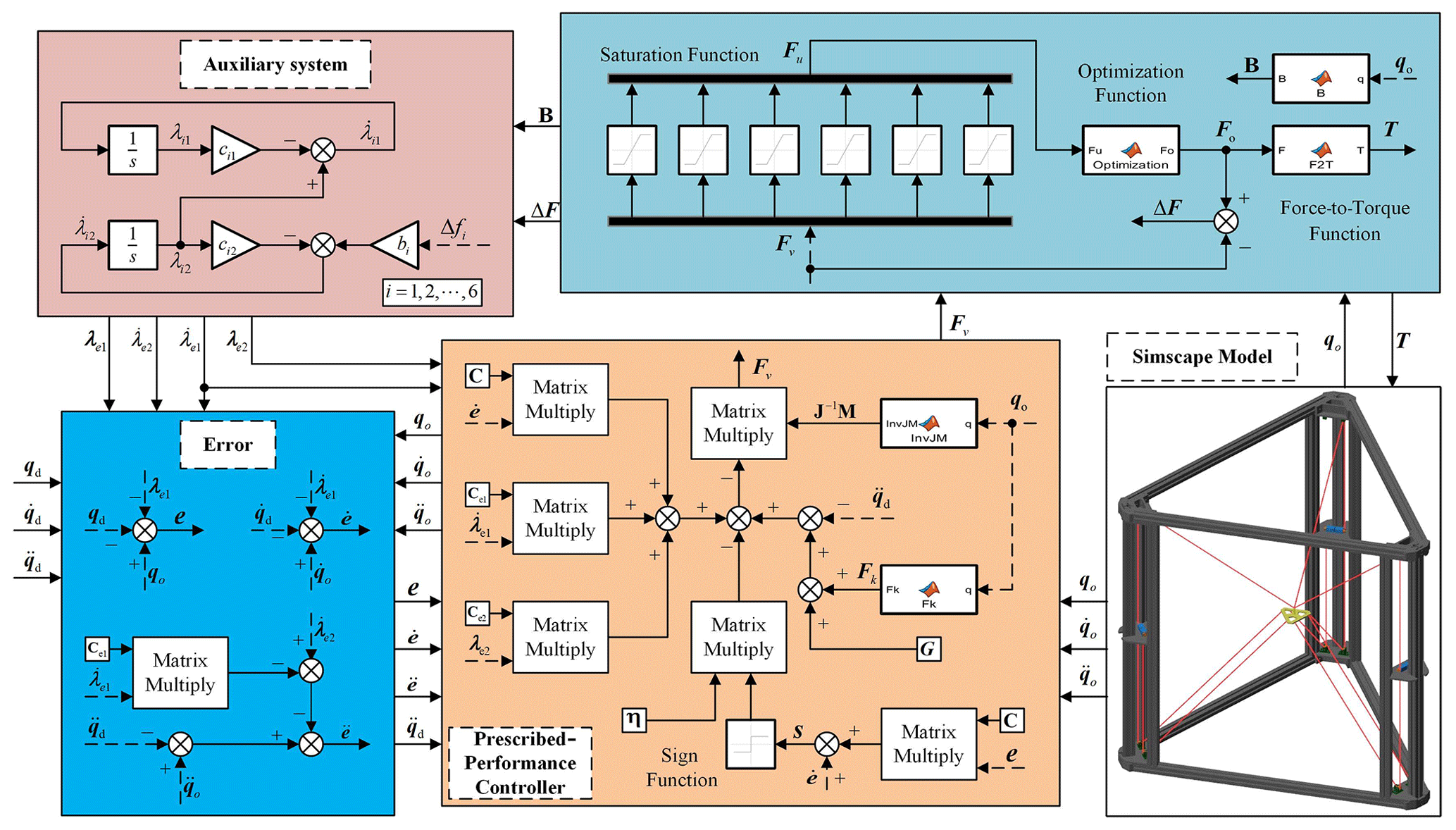
In order to validate the effectiveness of the prescribed-performance controller, a simulation model of the control system for the cable-driven 3D-printing motion platform is constructed in Simulink, as depicted in Fig. 9.

Figure 9 Prescribed-performance controller.

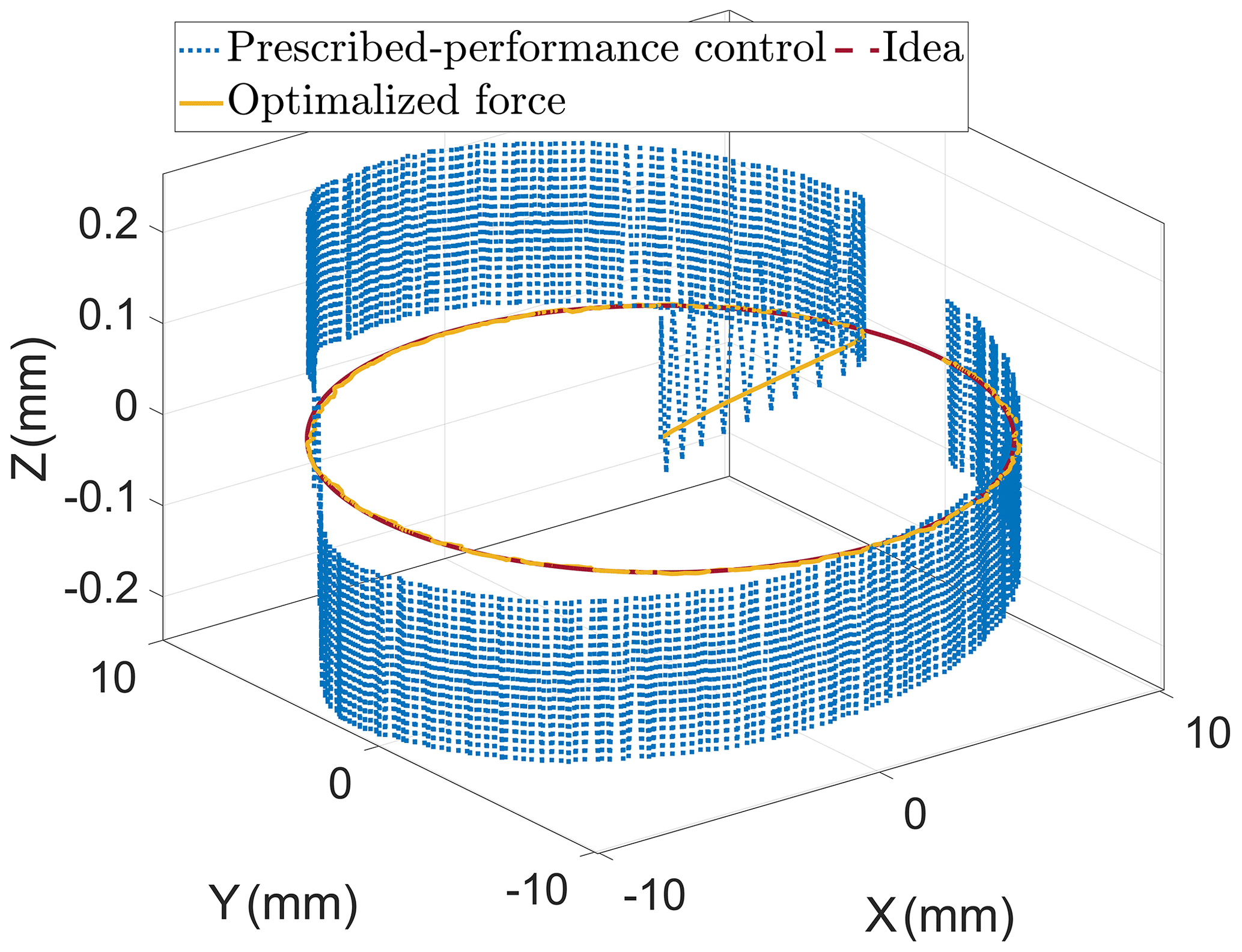
In the simulation, the trajectory expression of the end-effector is

$$\begin{array}{}\text{(35)}& \left\{\begin{array}{l}x=\mathrm{10}\cos \left(\mathrm{0.2}\mathit{\pi }t\right)\\ y=\mathrm{10}\sin \left(\mathrm{0.2}\mathit{\pi }t\right)\\ z=\mathrm{0}\end{array}\right.(\mathrm{0}\le t<\mathrm{10}).\end{array}$$

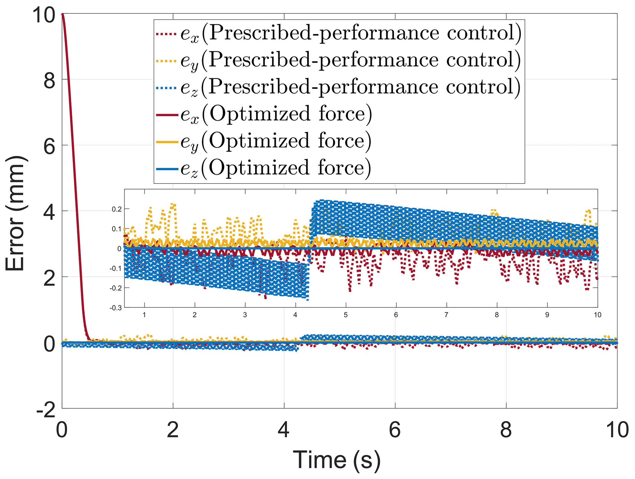
Figure 10 shows the corresponding 3R3T end-effector trajectory. As shown in Fig. 11, the maximum X-axis error ${∥e_x∥}_{\mathrm{\infty }}=\mathrm{0.259}$ mm, the maximum Y-axis error ${∥e_y∥}_{\mathrm{\infty }}=\mathrm{0.228}$ mm, and the maximum Z-axis error ${∥e_z∥}_{\mathrm{\infty }}=\mathrm{0.264}$ mm when using only the prescribed-performance controller. After cable force optimization, the maximum X-axis error ${∥e_x∥}_{\mathrm{\infty }}=\mathrm{0.040}$ mm, the maximum Y-axis error ${∥e_y∥}_{\mathrm{\infty }}=\mathrm{0.047}$ mm, and the maximum Z-axis error ${∥e_z∥}_{\mathrm{\infty }}<\mathrm{0.001}$ mm. The simulation results show that the controller with force optimization can reduce the X-axis error by 84.556 %, the Y-axis error by 79.386 %, and the Z-axis error by 99.962 %.

Figure 10 Trajectories of the end-effector in the controller simulation.

Figure 11 Errors of the end-effector in the controller simulation.

5 Experiment

5.1 Design of the experimental prototype

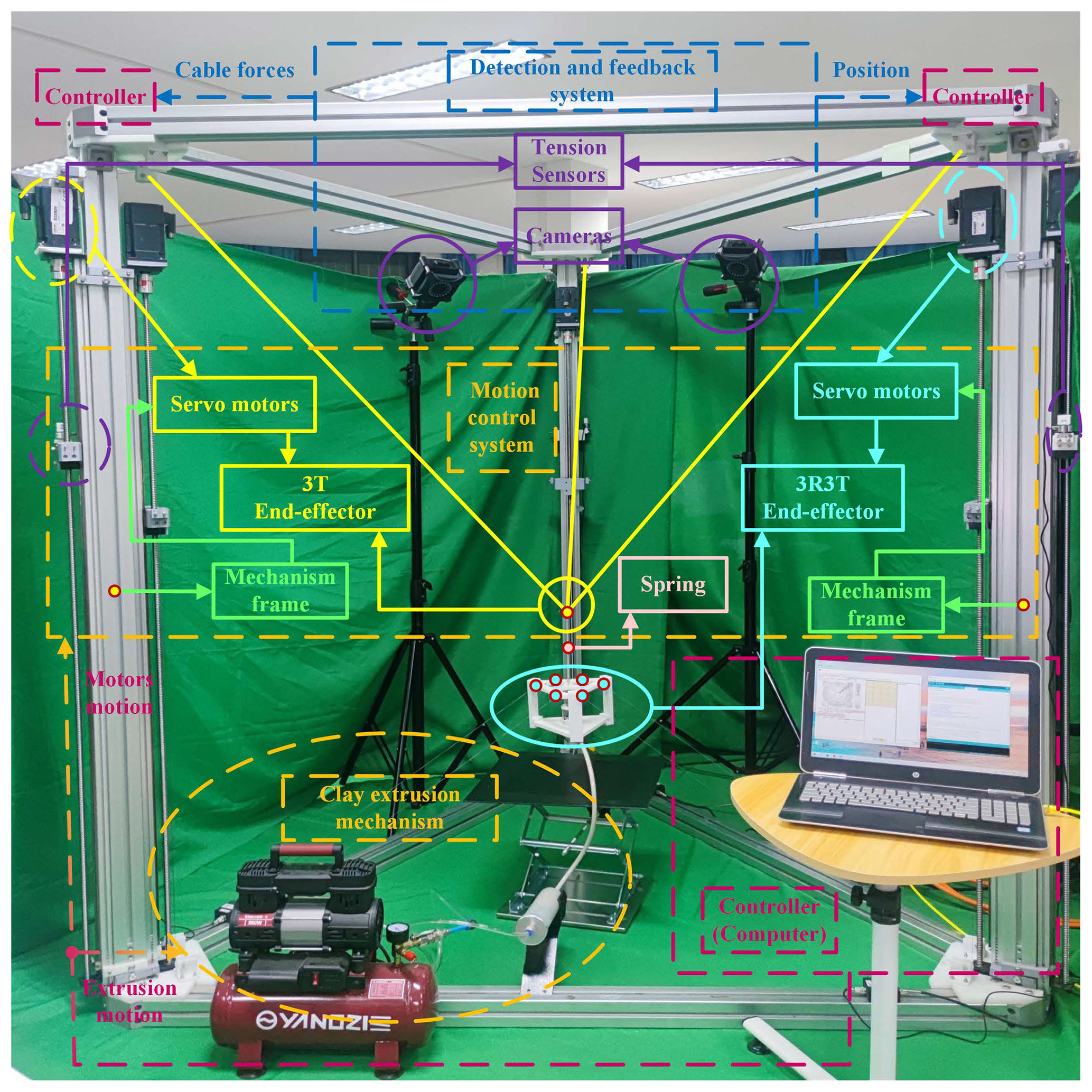
As depicted in Fig. 12, the cable-driven hybrid robot prototype consists of a motion drive system, a detection feedback system, and a clay extrusion mechanism. The motion drive system utilizes Beckhoff's C6650-0050 IPC and AX5201 driver to drive six AM8031 servo motors. The servo motors drive the cable through the screw and slider to enable precise control of the end-effector's movement. The motion control of the servo motors employs TwinCat3 software. The detection feedback system includes both force feedback and position feedback. Force feedback is obtained using Beckhoff's EL3064 digital analogue acquisition module to capture signals from the tension sensors, while the TE1410 module ensures synchronous signal transmission between TwinCat3 and Simulink. Position feedback is achieved using the NOKOV optical 3D motion capture system, which captures the end-effector’s position information. The captured data are then transferred to Simulink via the Software Development Kit (SDK) in a unidirectional manner. The extrusion mechanism consists of a constant-pressure air compressor and an extrusion nozzle.

Figure 12 Experimental prototype.

5.2 Error compensation experiment

According to the theoretical derivation and simulation calculation in Sect. 2, the trajectories shown in Eq. (15) are run five times with and without error compensation. Figure 13 illustrates the trajectories both with and without error compensation. Based on the sampling points in each trajectory, we calculate the plane error $e_r=\sqrt{x_d^{\mathrm{2}}+y_d^{\mathrm{2}}}-\sqrt{x_r^{\mathrm{2}}+y_r^{\mathrm{2}}}$, the mean plane error ${\stackrel{\mathrm{‾}}{e}}_r$, the plane error variance s_r, the maximum plane error e_rmax, the mean maximum plane error ${\stackrel{\mathrm{‾}}{e}}_{rmax}$, and the maximum plane error sample variance s_rmax for each trajectory. Based on the sampling points in each trajectory, we calculate the height error $e_{\mathrm{h}}=z_d-z_r$, the mean height error e_h, the variance of the height error ${\stackrel{\mathrm{‾}}{e}}_{\mathrm{h}}$, the maximum height error s_h, the mean maximum height error ${\stackrel{\mathrm{‾}}{e}}_{\mathrm{hmax}}$, and the sample variance of the maximum height error s_hmax for each trajectory. Figure 14a shows the plane error with the maximum point (P1–P6) of error, and Fig. 14b shows the height error with the maximum point (P1–P6) of height error.

Figure 13 Trajectories of the end-effector in the error compensation experiment

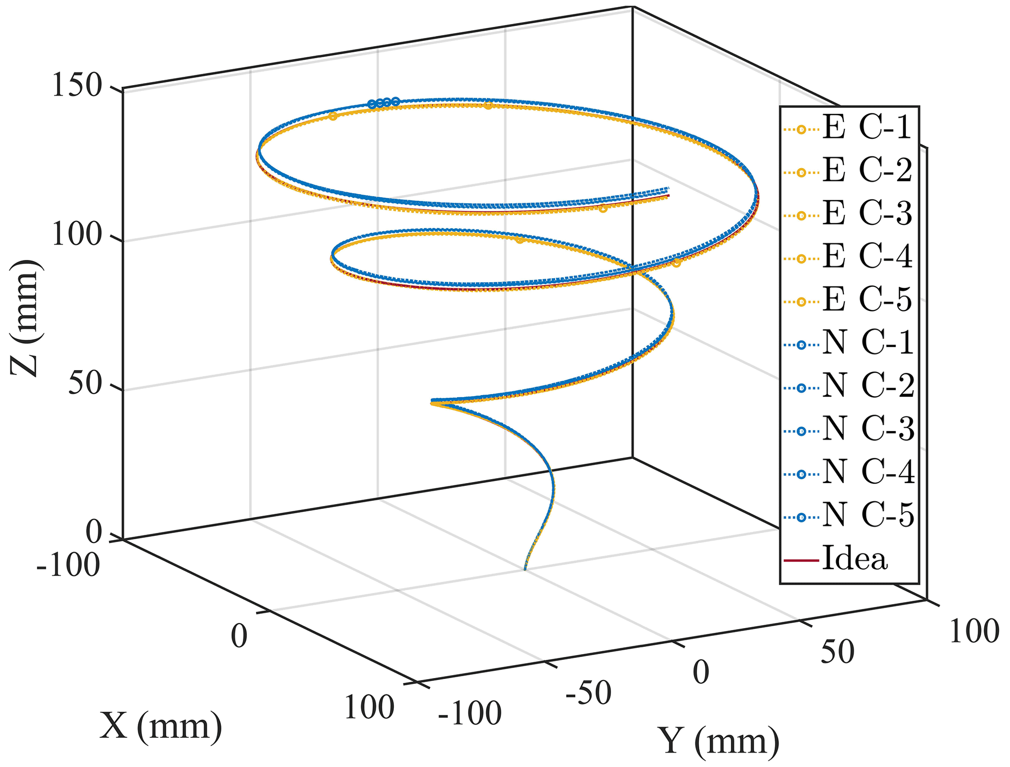
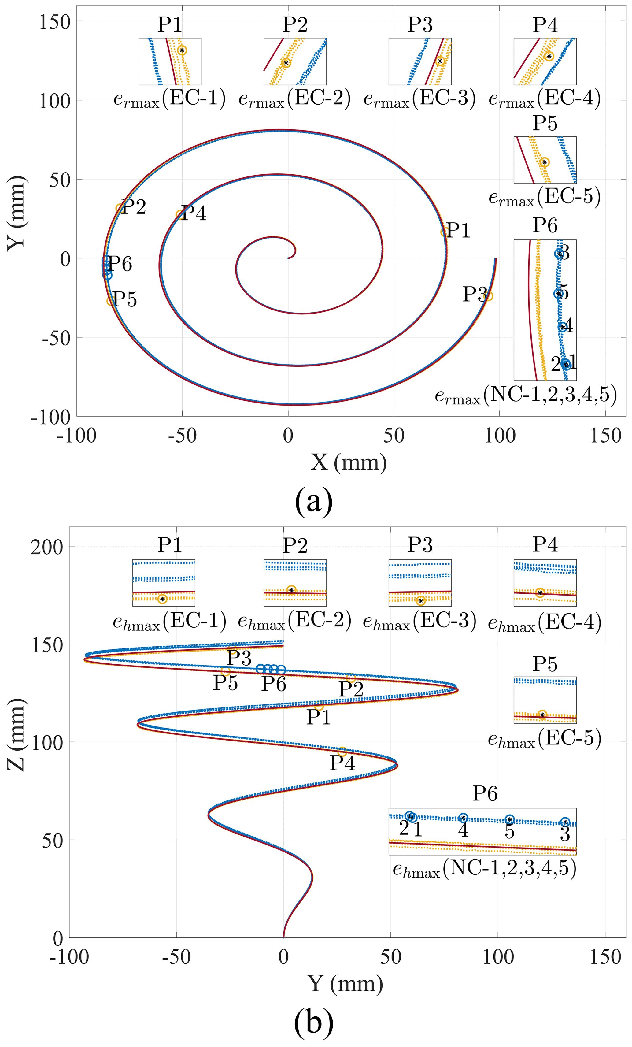
Figure 14 Error compensation experiment. (a) Plane trajectories of end-effector. (b) Height trajectories of end-effector.

According to Table 1, when there is non-compensation, the plane errors generated by running end-effector movements five times fluctuate around 0.733 mm, with variance greater than 0.14 and less than 0.2. The maximum plane errors are 1.590, 1.660, 1.623, 1.679, and 1.169 mm. The mean value of the maximum plane error is 1.636 mm, and the sample variance is $\mathrm{1.201}\times {\mathrm{10}}^{-\mathrm{3}}$. After the error compensation, the plane errors generated by running the end-effector movements five times fluctuate around 0.010 mm, with a variance greater than 0.015 and less than 0.02. The maximum plane errors are 0.361, 0.356, 0.364, 0.334, and 0.352 mm. The mean value of the maximum plane error is 0.353 mm, and the sample variance is $\mathrm{1.364}\times {\mathrm{10}}^{-\mathrm{4}}$. The mean value of the maximum plane error after error compensation is reduced by 78.395 % compared to non-compensation.

Table 1 Plane errors and height errors in the error compensation experiment (mm).

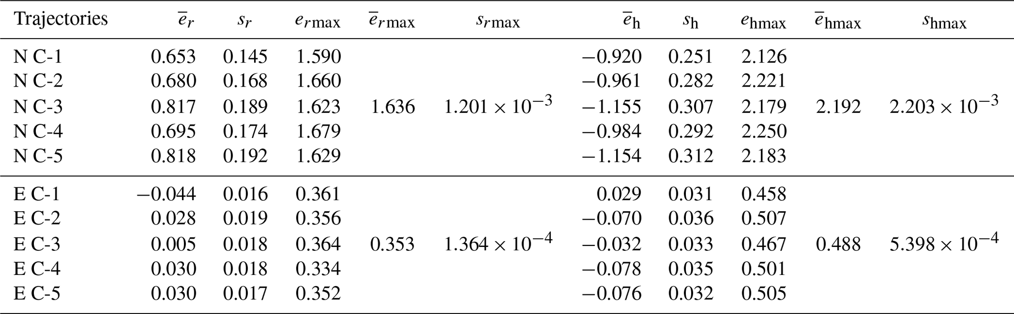
According to Table 1, when there is non-compensation, the height errors generated by running the end-effector movements five times fluctuate around −1.035 mm, with variance greater than 0.25 and less than 0.32. The maximum plane errors are 2.126, 2.221, 2.179, 2.250, and 2.183 mm. The mean value of the maximum plane error is 2.192 mm, and the sample variance is $\mathrm{2.203}\times {\mathrm{10}}^{-\mathrm{3}}$. After the error compensation, the height errors generated by running the end-effector movements five times fluctuate around −0.045 mm, with a variance greater than 0.03 and less than 0.035. The maximum plane errors are 0.458, 0.507, 0.467, 0.501, and 0.505 mm. The mean value of the maximum plane error is 0.488 mm, and the sample variance is $\mathrm{5.398}\times {\mathrm{10}}^{-\mathrm{4}}$. The mean value of the maximum plane error after error compensation is reduced by 77.755 % compared to non-compensation.

5.3 Prescribed-performance controller experiment

According to the results of the experiment (Sect. 5.2), the error compensation can effectively reduce the plane error and height error in the open-loop control. Therefore, to investigate the control accuracy of the preset performance controller in a larger plane area, the end-effector motion radius is increased from 98.299 mm in the experiment (Sect. 5.2) to 185.887 mm, and the motion trajectory is

$$\begin{array}{}\text{(36)}& \left\{\begin{array}{l}x={\ln }^{\mathrm{3}}\left(\mathrm{2}t+\mathrm{1}\right)\cos \left(\frac{\mathit{\pi }}{\mathrm{75}}t\right)\\ y={\ln }^{\mathrm{3}}\left(\mathrm{2}t+\mathrm{1}\right)\sin \left({\displaystyle \frac{\mathit{\pi }}{\mathrm{75}}}t\right)\\ z=\mathrm{0}\end{array}\right.(\mathrm{0}\le t<\mathrm{150}).\end{array}$$

The motion trajectories on the open-loop control with and without radius compensation and the prescribed-performance controller are shown in Fig. 15. The plane error and height error are shown in Fig. 16a–b.

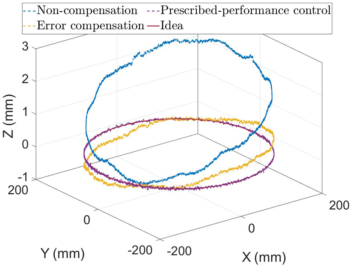
Figure 15 Trajectories of the end-effector in the prescribed-performance controller experiment.

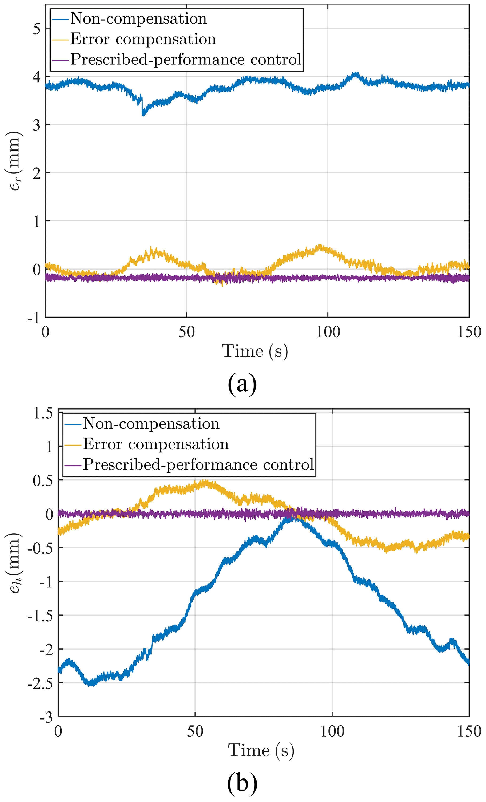
Figure 16 Prescribed-performance controller experiment. (a) Plane errors of end-effector. (b) Height errors of end-effector.

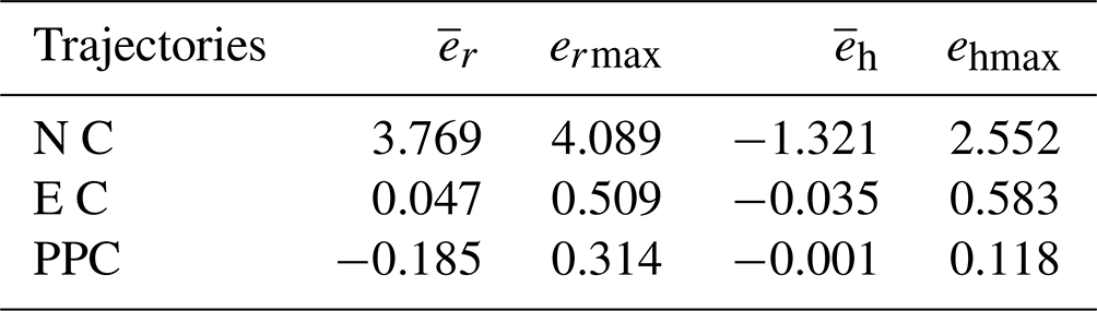
As shown in Table 2, the maximum plane error with non-compensation is 4.089 mm, and the maximum plane error after error compensation is 0.509 mm, which is reduced by 87.552 %. The maximum plane error of the preset-sliding-mode controller is 0.314 mm, which is reduced by 92.321 %. The maximum height error with non-compensation is 2.552 mm, and the maximum plane error after error compensation is 0.583 mm, which is reduced by 77.155 %. The maximum plane error of the prescribed-performance controller is 0.118 mm, which is reduced by 95.376 %.

Table 2 Plane errors and height errors in the prescribed-performance controller experiment (mm).

Figure 17 Clay-printing experiment.

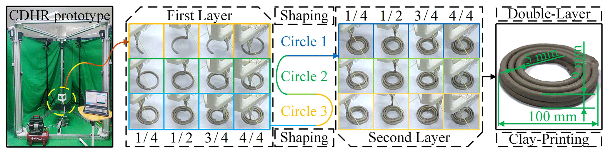
5.4 Clay-printing experiment

In order to ascertain the feasibility of the mechanisms, a clay-printing experiment was conducted using the CDHR prototype. The clay is conveyed to the extrusion mechanism using a constant air pressure of 0.2 MPa. The extrusion diameter measures 5 mm. As shown in Fig. 17, the results of the double-layer printing show consistent and uniform clay diameter, accurate formation, and precise alignment between the start and end points. Furthermore, the experimental results demonstrate that the thickness of each clay layer printed is consistent.

6 Conclusions

In this paper, a 3-DOF cable-driven hybrid 3D-printing mechanism is proposed. A vector analysis method is proposed to compensate for errors in kinematics, dynamics, and cable force analysis for this mechanism. The effect of the pulley systems on the motion error of the end-effector is analysed. A physical simulation environment of the mechanism is established using Simscape. The correctness of the proposed vector analysis method and the effectiveness of the error compensation are verified in the physical simulation environment. A prescribed-performance controller for multi-input, multi-output (MIMO) nonlinear systems is proposed based on the cable characteristics. The output cable force of the controller is optimized to meet the strict accuracy requirement of the end-effector motion. The effectiveness of the controller in improving motion accuracy and stability is verified using the physical simulation environment.

An experimental prototype of a 3-DOF cable-driven hybrid 3D-printed mechanism is proposed and constructed. The error compensation verification experiments were designed based on the vector analysis method, comparing the results with and without error compensation. The experimental results indicated that, compared to non-compensation, the mean value of the maximum plane error after error compensation is reduced by 78.395 %, and the mean value of the maximum height error after error compensation is reduced by 77.755 %. The prescribed-performance controller experiment is conducted based on the prescribed-performance controller. The experimental results show that, with error compensation, the maximum plane error is reduced by 87.552 %, the maximum plane error of the prescribed-performance controller is reduced by 92.321 %, the maximum height error is reduced by 77.155 %, and the maximum height error of the prescribed-performance controller is reduced by 95.376 % compared to non-compensation. Finally, the results of the double-layer clay-printing experiment illustrate that the CDHR mechanism is feasible.

Appendix A: Parameter values

Table A1 The values of Parameters.

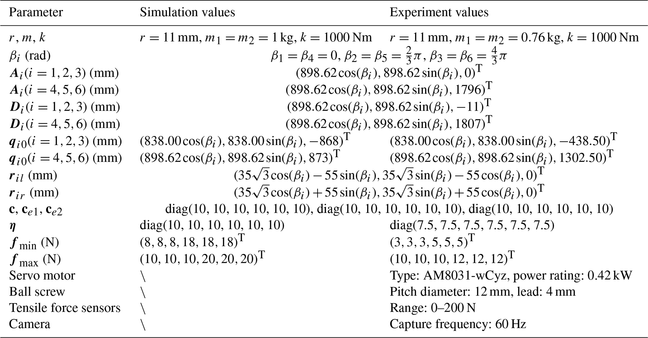
\ indicates that the parameter is not involved in the simulation.