Numerical and experimental investigation of the effect of process parameters on sheet deformation during the electromagnetic forming of AA6061-T6 alloy

Electromagnetic forming is a high-speed sheet metal forming technique to form metallic sheets by applying magnetic forces. In comparison to the conventional sheet metal forming process, electromagnetic forming is a process with an extremely high velocity and strain rate, which can be effectively used for the forming of certain difficult-to-form metals. During electromagnetic forming, it is important to recognise the effects of process parameters on the deformation and sheet thickness variation of the sheet metal. This research focuses on the development of a numerical model for aluminium alloy (AA6061-T6) to analyse the effects of three process parameters, namely voltage, sheet thickness and number turns of the coils, on the deformation and thickness variation of the sheet. A two-dimensional fully coupled finite-element (FE) model consisting of an electrical circuit, magnetic field and solid mechanics was developed and used to determine the effect of changing magnetic flux and system inductance on sheet deformation. Experiment validation of the results was performed on a 28 KJ electromagnetic forming system. The Taguchi orthogonal array approach was used for the design of experiments using the three input parameters (voltage, sheet thickness and number of turns of the coil). The maximum error between numerical and experimental values for sheet thickness variation was observed to be 4.9 %. Analysis of variance (ANOVA) was performed on the experimental results. Applied voltage and sheet thickness were the significant parameters, while the number of turns of the coil had an insignificant effect on sheet deformation. The contribution ratio of voltage and sheet thickness was 46.21 % and 45.12 % respectively. The sheet deformation from simulations was found to be in good agreement with the experimental results.

1 Introduction

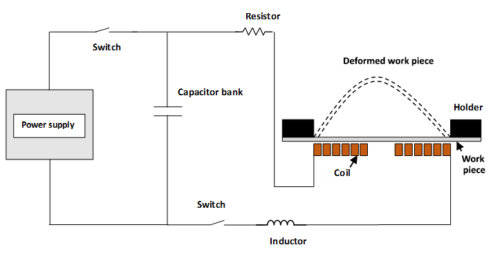
Electromagnetic forming, also known as a high-velocity forming process, involves deformation of the metallic sheet under the influence of magnetic forces. The repulsive forces between conducting coil and workpiece are generated by mutual inductance that creates opposing magnetic fields and Lorentz forces acting on conducting bodies. A simplified schematic diagram of electromagnetic forming is shown in Fig. 1.

Figure 1 Schematic of the electromagnetic forming process for Al 6061-T6.

Electromagnetic forming is increasingly finding its application in sheet metal forming for the automotive, appliance, aerospace and other fields due to its effectiveness in forming aluminium and other low-formability materials (Psyk et al., 2011). Due to high-speed deformation, the formability of the material can be increased by electromagnetic forming, and the phenomena of wrinkling and spring back can be minimized. Numerical simulations have always attracted the interest of researchers as it is not feasible to find out optimum parameters for every metal and die shape experimentally. Numerical methods have therefore been used to determine the suitable parameters before physically forming a sheet (El-Azab et al., 2003). Experiments on free bulging of an annealed aluminium disk and its numerical simulation were first conducted by Takatsu et al. (1988). The effects of magnetic field penetration into the disk and elastoplastic deformation were combined and taken into account. Spiral coil was represented as coaxial circular loops carrying discharge current. Fenton and Daehn also worked on a two-dimensional arbitrary Langrangian–Eulerian (ALE) model to develop a finite-difference code (CALE) to predict the deformation of sheet metal (Fenton and Daehn, 1998). The model required two different time steps to maintain the numerical stability of magnetic physics and material motion. This problem was resolved by Oliveira et al. (2005) by using a loose coupling method to analyse the dynamic behaviour of sheet metal. ANSYS/EMAG and LS DYNA were used, but the effect of change in geometry on the magnetic field was not considered, which resulted in overestimation of sheet deformation. Correia et al. (2008) used commercial finite-element code in ABAQUS/Explicit to study the deformation of sheet and influence of visco-plastic material behaviour in the free bulge electroforming process, neglecting the effect of velocity. This model was simpler and easy to implement because electromagnetic forces were calculated and then used as body load in the sheet deformation process. Therefore, the simulation results also showed overestimation of sheet deformation in comparison to the experimental results. Haiping et al. (2009) presented a more realistic model. They worked on a sequential coupled field model for the electromagnetic tube forming process. The effect of change in geometry on the magnetic force was taken into consideration, but the change in the inductance of the workpiece and circuit was ignored. This model was also limited to axisymmetric problems. Cui et al. (2011) also worked on a sequential coupled model by incorporating adaptive remeshing technique remeshing the air continuously as the sheet deforms. This model was, however, limited to two-dimensional axisymmetric problems. Li et al. (2013) used ANSYS/EMAG to calculate Lorentz force on a rigid sheet and then imported the forces to ABAQUS/Explicit software for three-dimensional deformation analysis. However, the model was uncoupled. A fully coupled model for axisymmetric free bulging of aluminium alloy was developed by Cao et al. (2014). The effect of velocity on the current applied to the coil was considered. The results of the fully coupled numerical model were compared with the experimental work of Takatsu et al. (1988). Simulated deformation of Cao et al. (2014) gave much improved results than the previous uncoupled models. However, sequential coupling increases the simulation time and complicates the model, making it difficult to converge, which is advisable for axisymmetric problems. Yu et al. (2018) discussed the comparison of conventional forming and electromagnetic forming. Circular hole flanging by electromagnetic forming showed better formability compared to conventional forming. The uncoupled three-dimensional numerical model was in good agreement with experimental results. Similarly, Noh et al. (2014) performed experiments and uncoupled three-dimensional numerical simulations for sheet metal forming with an unsymmetrical die. A loosely coupled FE model was used to analyse the operational parameters of the electromagnetic forming process to better understand its industrial applications. The deformation of the workpiece was neglected in the FE model to reduce computational time (Mamalis et al., 2006), but to get better results, the fully coupled model should be used. Another sequential FE model was developed to compare and analyse deformation of ribbed sheets with plane sheets (Lei et al., 2017). The ribbed sheets undergo larger force because of larger skin depth. The maximum value of force was very close for the x–y grid and plane sheet. Ribbed sheet showed better deformation as compared to plane sheet. Sequential coupling gave better results as compared with loose coupling.

An experimental study was carried out by Huang et al. (2019) where a controlled pulsed electromagnetic blank holder system was fabricated and tested. With this method, the wrinkling of the edges was reduced, and the flow of flange and deformation behaviour was improved.

In this research, a fully coupled numerical model was developed to predict closed die sheet metal electromagnetic forming. The model consists of an electrical circuit module coupled with a magnetic field module to generate the required pulsed current to the coil. A solid mechanics module was also coupled with a magnetic field module to get the instantaneous value of inductance. The change in magnetic field and current density with changing geometry was also considered. Experiments were conducted for comparison and to validate the numerical model. Numerical simulations and experiments were carried out by varying three process parameters, i.e. input voltage, sheet thickness and number of turns of the coil. Numerical results of the difference between the die and sheet being deformed (ΔX_average) were compared with experimental results. The effects of sheet thickness variation at various points along the sheet were also compared with the experimental results. The significance and contribution ratio of each parameter were also calculated.

Figure 2 RLC equivalent circuit of the EMF process.

2 Equivalent circuit

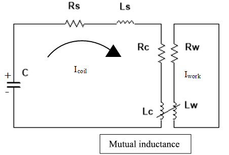
The electrical equivalent circuit of electromagnetic forming is shown in Fig. 2. R_s and L_s are system resistance and inductance. R_c and R_w are coil and workpiece resistance, while L_s and L_w are coil and workpiece inductance. M is the mutual inductance which depends on the coupling factor. The coupling factor decreases with an increase in the workpiece and coil gap (Dond et al., 2018). By increasing the coil and workpiece gap, the magnetic pressure decreases, which is not desirable. Therefore, in this research, the gap has been kept constant throughout the experiments and simulations. The limiting value experimentally is 2 mm, while simulation of the 1 mm gap is also available in the literature (Dond et al., 2018). The total equivalent resistance and inductance of a coupled system can be written as follows (Mamalis et al., 2004).

$$\begin{array}{}\text{(1)}& {\displaystyle }L=L_{\mathrm{s}}+L_{\mathrm{c}}-{\displaystyle \frac{M^{\mathrm{2}}}{L_{\mathrm{w}}}}\text{(2)}& {\displaystyle }R=R_{\mathrm{s}}+R_{\mathrm{c}}+{\displaystyle \frac{M^{\mathrm{2}}}{{L_{\mathrm{w}}}^{\mathrm{2}}{R}_{\mathrm{w}}}}\text{(3)}& {\displaystyle }M=K\sqrt{L_{\mathrm{C}}{L}_{\mathrm{w}}}\end{array}$$

K is the coupling factor between coil and workpiece. K is kept constant in this case. By keeping the workpiece coil gap constant, we can keep inductance (L), resistance (R), coil current (I(t)), damping coefficient (β), and frequency (ω) of the system constant (Dond et al., 2018).

$$\begin{array}{}\text{(5)}& {\displaystyle }I\left(t\right)={\displaystyle \frac{U_{\mathrm{0}}}{\mathit{\omega }L}}{e}^{-\mathit{\beta }t}\sin \left(\mathit{\omega }t\right)\text{(6)}& {\displaystyle }\mathit{\beta }={\displaystyle \frac{R}{\mathrm{2}L}}\text{(7)}& {\displaystyle }\mathit{\omega }=\sqrt{{{\displaystyle \frac{\mathrm{1}}{L}}}_{\mathrm{C}}-{\mathit{\beta }}^{\mathrm{2}}}\end{array}$$

3 Numerical modelling

The numerical model consists of three modules: (a) electrical circuit; (b) electromagnetic field; (c) solid mechanics. All three modules are fully coupled in the time-dependent study.

3.1 Electrical circuit

The electrical circuit as discussed earlier is an RLC circuit with a power bank and two terminals that are connected to the coil. The input parameters for the electrical circuit are resistance of the system (R_s), inductance of the system (L_s), voltage (U₀), and capacitance of the capacitor bank (C). The model executes time-dependent current Eq. (4) to calculate the damped alternating current. The current frequency is important for calculating skin depth (Singh and Mogi, 2003).

$$\begin{array}{}\text{(8)}& \mathit{\delta }=\sqrt{{\displaystyle \frac{\mathrm{2}}{\mathit{\sigma }\mathit{\mu }\mathit{\omega }}}},\end{array}$$

where δ is skin depth which varies with angular frequency (ω), magnetic permeability (μ) and half-space conductivity (σ) (Singh and Mogi, 2003). Frequency was kept constant and according to the sheet thickness.

3.2 Magnetic field

Electromagnetic equations involved in magnetic field model are as follows (Dond et al., 2018):

$$\begin{array}{}\text{(9)}& {\displaystyle }\mathrm{\nabla }xH=J,\text{(10)}& {\displaystyle }\mathrm{\nabla }xE={\displaystyle \frac{-\mathrm{d}B}{\mathrm{d}t}},\text{(11)}& {\displaystyle }\mathrm{\nabla }xB=\mathrm{0},\text{(12)}& {\displaystyle }J={\displaystyle \frac{I_{\mathrm{c}}}{\mathrm{s}}}={\mathit{\sigma }}_{\mathrm{e}}E,\end{array}$$

where H is magnetic intensity, J is current density, s is the sectional area of one turn of coil, B is magnetic flux density, E is electric intensity, and σ_e is electrical conductivity.

3.3 Solid mechanics module

When time-varying current flows through the coil, it produces eddy current in the nearby conducting coil; as a result, Lorentz forces are generated. Lorentz force between the coil and workpiece results in the deformation of the workpiece. The displacement equation for the workpiece is given by the equilibrium equation (Dond et al., 2018):

$$\begin{array}{}\text{(13)}& \mathit{\rho }{\displaystyle \frac{{\mathrm{d}}^{\mathrm{2}}\mathit{u}}{\mathrm{d}{t}^{\mathrm{2}}}}-\mathrm{\Delta }\mathit{\sigma }\mathrm{s}=\stackrel{\mathrm{‾}}{\mathrm{fm}},\end{array}$$

where ρ is density, u is the displacement vector, σs is the stress tensor and $\stackrel{\mathrm{‾}}{\mathrm{fm}}$ is the electromagnetic force density.

Figure 3 Mesh of EMF closed die for electromagnetic forming of Al 6061-T6.

Since electromagnetic forming is high-speed deformation, high strain rate effect on mechanical properties of the workpiece must be defined. Generally, there are three models majorly used for high-speed deformation (a) Steinberg model (Fenton and Daehn, 1998) Eq. (13), (b) Johnson–Cook model (Patil et al., 2017) Eq. (14) and (c) Cowper–Symonds constitutive model (Li et al., 2013) Eq. (15).

$$\begin{array}{}\text{(14)}& {\displaystyle }\mathit{\sigma }=\mathrm{93}.(\mathrm{1}+\mathrm{125}\mathit{\epsilon }{)}^{\mathrm{0.1}}\text{(15)}& {\displaystyle }\mathit{\sigma }=\left[A+B{\left(\mathit{\epsilon }\right)}^n\right]\left[\mathrm{1}+\text{Cln}\left(\dot{\stackrel{\mathrm{‾}}{\mathit{\epsilon }}}\right)\right]\text{(16)}& {\displaystyle }\stackrel{\mathrm{‾}}{\mathit{\sigma }}={\mathit{\sigma }}_y\left[\mathrm{1}+{\left({\displaystyle \frac{\dot{\stackrel{\mathrm{‾}}{\mathit{\epsilon }}}}{p}}\right)}^m\right]\end{array}$$

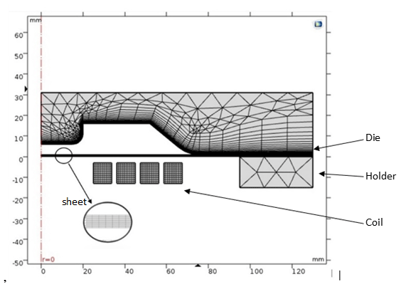
In the current research, the Cowper–Symonds model was used for closed die sheet metal forming. The model is relatively simple as it uses only three material constants, while the Johnson–Cook model requires five material parameters. The results fit well with experimental data (Al Salahi and Othman, 2016). Meshing of the electromagnetic forming process is shown in Fig. 3. The die and holder were rigid during solid mechanics simulation in which only deformation of the sheet is analysed. The coil was only included in magnetic field generation and was excluded from the solid mechanics model to reduce simulation time. The sheet domain was included in the magnetic field and the solid mechanics model because it will be subjected to both magnetic field-induced Lorentz force as well as deformation. Mesh convergence was carried out using the iterative method. Mapped mesh was used for the coil and the sheet. Boundary meshing was used for the die. Tetrahedral meshing was used for the surrounding air and blank holder. Surrounding air was considered in magnetic field generation as the deforming mesh. Moving mesh was not required for the air domain since it was not included in solid mechanics non-linear analysis. The complete mesh consisted of 5020 domain elements and 534 boundary elements.

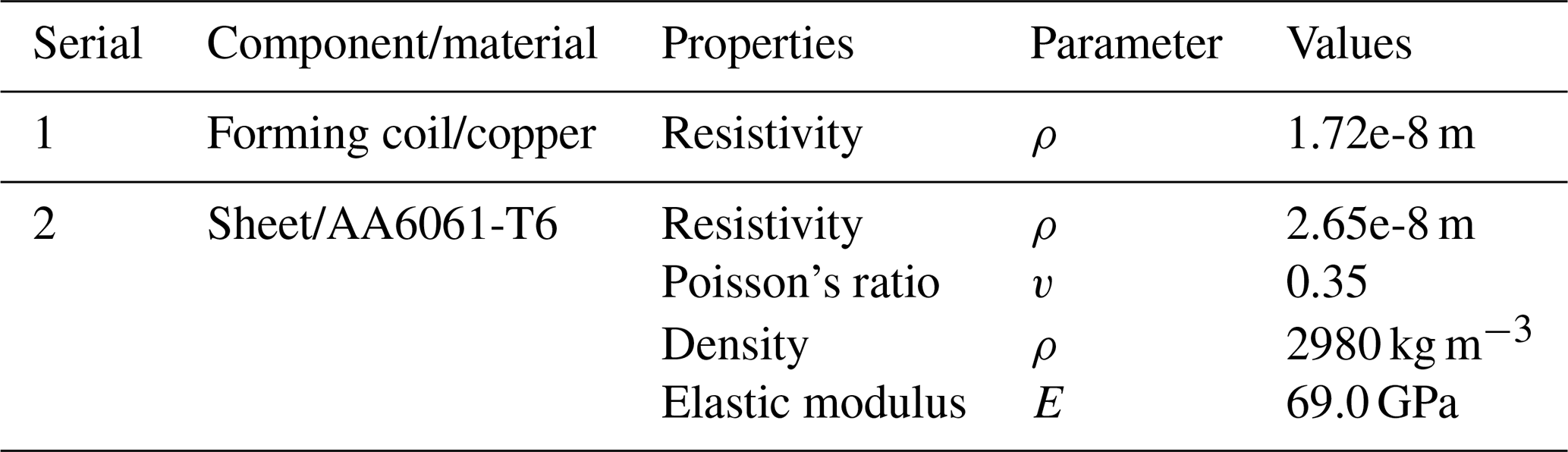
The electrical and mechanical properties of the sheet and constants for the model were taken from the work of Cui et al. (2014), where the constants used were p=6500 s⁻¹ and m=0.25. For simulation of Sheet/AA6061-T6, the Cowper–Symonds model Eq. (15) was used. Properties are given below in Table 1.

Table 1 Electrical and mechanical properties of the sheet and coil (Cui et al., 2014).

3.4 Numerical model flow chart

A finite-element (FE) model was used to numerically solve the two-dimensional differential equations detailed above. The flow chart for the overall simulation process is shown in Fig. 4. In the simulation, discharge current flowing through the coil was calculated by solving Eq. (4). Magnetic flux and current density were calculated using Eqs. (8)–(11). The magnetic force was then calculated using Eq. (12). The deformation of the workpiece was calculated in solid mechanics which use magnetic force as a body load on the sheet. Initial parameters of the electromagnetic forming process were defined in the COMSOL^® Multiphysics software. An electrical circuit was designed in the electrical circuit module to generate a high ampere damped current. Two-dimensional geometry consisted of five domains. Coil domain was related to the current source that was generated in the electrical circuit module. The remaining four domains were sheet domain, die domain, air domain and blank holder domain. A magnetic field module was used to get the required Lorentz forces. The magnetic field module was fully coupled with the solid mechanics module to get the instantaneous deformation of the sheet with changing Lorentz forces with respect to time. A time-dependent study was used in the simulations.

Figure 4 Flowchart of the finite-element method.

Figure 5 Schematic of the electromagnetic forming system.

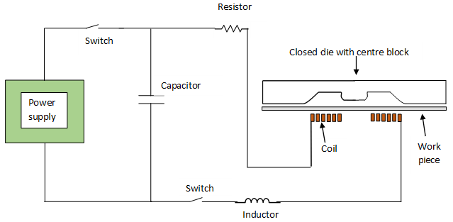
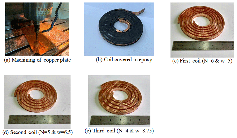
Figure 6 (a) Manufacturing of the coil on the CNC milling machine and (b) coil gap covered in epoxy. (c–e) Varying sizes of coils used in the experimentation.

4 Experimental setup

The schematic of the electromagnetic forming system with a closed die sheet metal forming arrangement is given in Fig. 5. The setup consisted of a power supply which can provide input voltage (U₀) ranging from 400 to 3000 V connected to a capacitor bank through a switch. The capacitor bank that was used in the experiments had a capacitance (C) of 6e-3F. Resistance (R) of 0.02 Ω and inductance (L) of 1.5e-6H of the RLC circuit were connected in series with the capacitor bank. The ends of the RLC circuit were connected with a spiral coil which was also completely covered with epoxy. The workpiece was held tightly between the die and coil.

Figure 7 Drawing of the die used in experimentation.

Figure 8 Die used in experimentation for electromagnetic forming of the Al 6061-T6 alloy.

4.1 Design of experiments

A Taguchi L9 array was used to study the effect of input parameters on the average difference between the sheet and die profile (ΔX_average) and the thickness of deformed sheets. Table 2 shows all the parameters and their levels. Generally, sheet thicknesses used in automotive parts vary from 0.5 to 2 mm. Most of the automobile industries use a sheet of gauge 20 in small vehicles and gauge 16 in large vehicles. For example, external panels such as roof, hood, and door have thicknesses of around 0.6 to 0.9 mm. The parts located beneath the car body such as supports, amplifiers, and flanges are 1.5–2.5 mm thick (Hovorun et al., 2017). The suitable range of voltage and number of turns of the coil were selected from the literature corresponding to the sheet thickness of 1 to 2 mm (Noh et al., 2014).

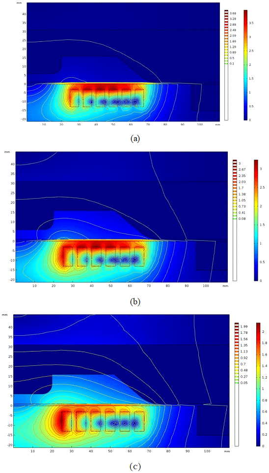
Figure 9 (a) Magnetic field at time step 100 µs (voltage = 2400, sheet = 1.02 mm, N=6). (b) Magnetic field at time step 190 µs (voltage = 2400, sheet = 1.02 mm, N=6). (c) Magnetic field at time step 315 µs (voltage = 2400, sheet = 1.02 mm, N=6).

Table 2 Taguchi L9 array for electromagnetic forming of the Al 6061-T6 alloy.

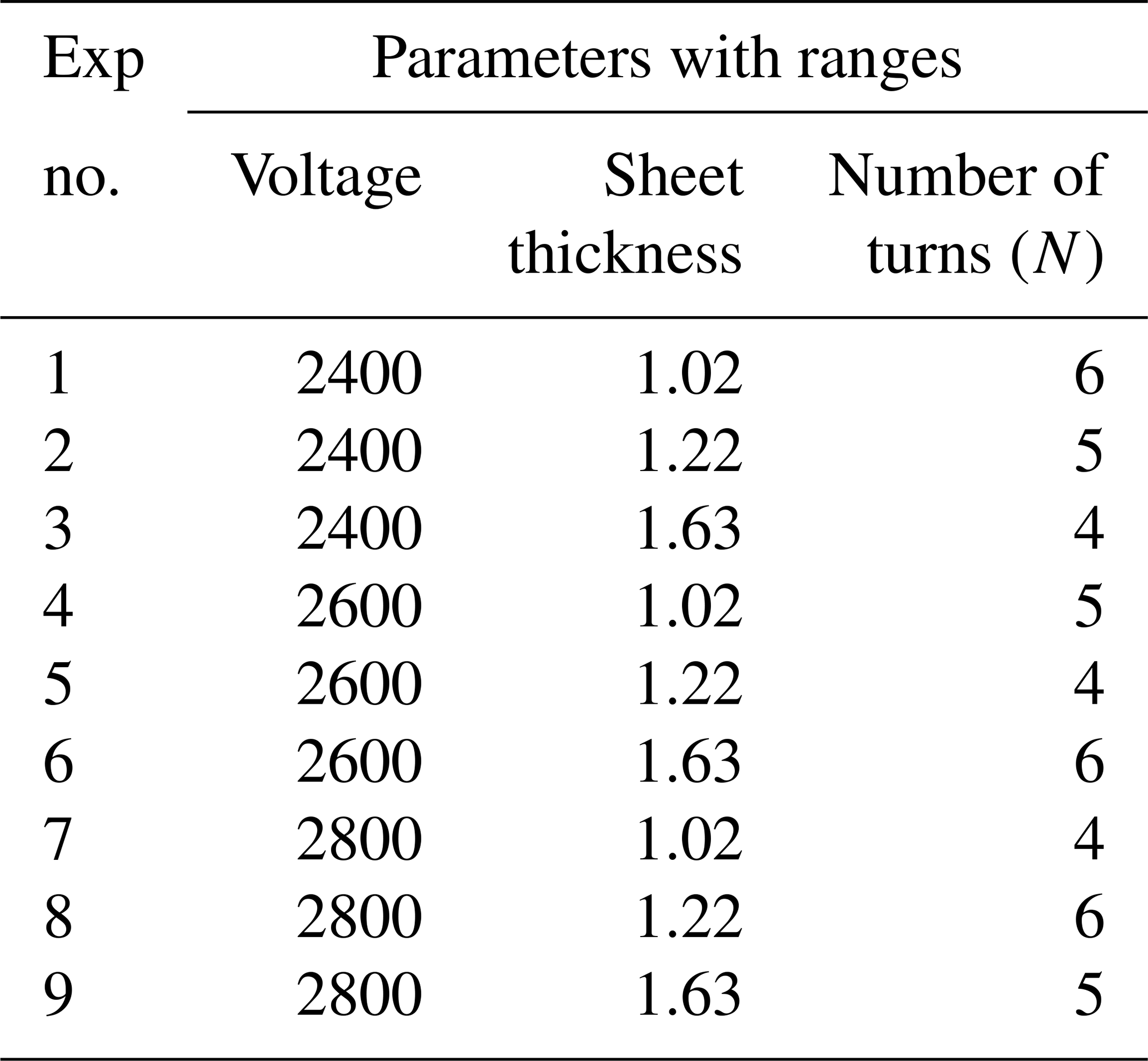
Figure 10 Maximum Lorentz force values for all conditions obtained from numerical simulation.

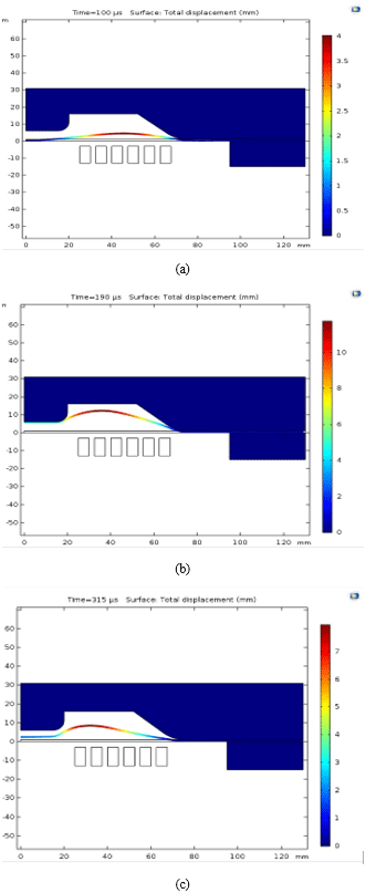
Figure 11 Total displacement at various time steps: (a) time step 100 µs (voltage = 2400, sheet = 1.02 mm, N=6), (b) time step 190 µs (voltage = 2400, sheet = 1.02 mm, N=6), (c) time step 315 µs (voltage = 2400, sheet = 1.02 mm, N=6).

4.2 Coils and die preparation

Copper coils used in the experiments were machined on three-axis CNC milling with an automatic 24-tool changer. (Max size: $\mathrm{600}\times \mathrm{600}\times \mathrm{1000}$ mm; maximum rpm 4000). Coil parameters are mentioned in Table 3.

Table 3 Coil parameters used in the experimentation.

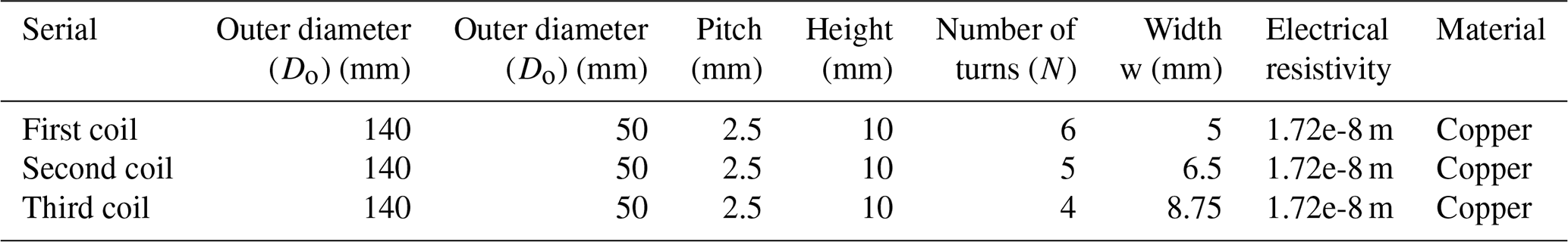
The electrical resistivity of the coil was measured by passing a known current through the rectangular cross-sectional coil and by measuring the voltage drop across the coil. The electrical resistivity was calculated to be 1.72e-8 ohm-m. The gaps between the turns of the coil were filled with epoxy resin and kept in a supporting fixture to eliminate any structural changes during the forming process. The prepared coils are shown in Fig. 6.

Figure 12 Velocity profile investigated at four points on the deformed Al 6061-T6 sheet.

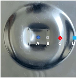
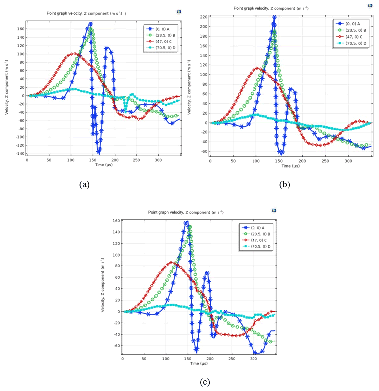
Figure 13 Velocity of four points on sheets. (a) Voltage = 2400 V, thickness = 1.02 mm, N=6. (b) Voltage = 2800 V, thickness = 1.22 mm, N=6. (c) Voltage = 2600 V, thickness = 1.63 mm, N=6.

Figure 14 Top view of deformed sheets. (a) Thickness = 1.02 mm, V = 2400, N=6. (b) Thickness = 1.22 mm, V = 2800, N=6. (c) Thickness = 1.63 mm, V = 2600, N=6.

4.3 Die preparation and sheet material selection

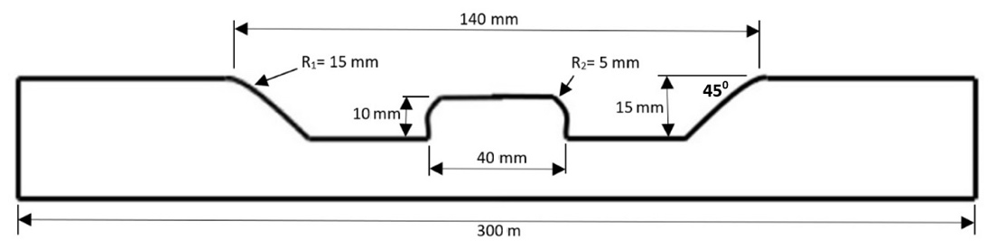
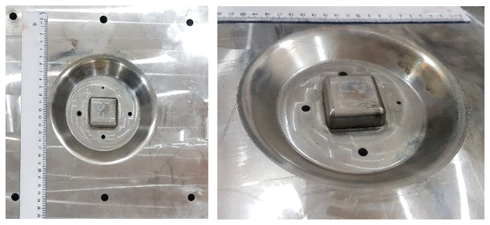
The closed die was machined using the CNC milling machine. The die was machined out of 300 mm × 300 mm × 40 mm non-magnetic stainless steel (austenitic 304). It had a central square block (40 mm × 40 mm) and air vents (4 mm diameter) to prevent air being entrapped between the sheet and die. It had six holes for bolting it onto the die-holding fixture. Cross-sectional drawing of the die is shown in Fig. 7, while the actual die manufactured and used in the experiments is shown in Fig. 8. The die used in this research is identical to the one reported by Noh et al. (2014) so as to evaluate the FE model. Due to the central block and intricate shape, the die has a pronounced spring back effect. This geometry is also suitable for predicting how well the FE model behaves in sharp curves and edges.

Aluminium alloy (AA6061-T6) sheets were considered for experimentation in this research. The thickness range for the Standard Wire Gauge (SWG) was 16, 18 and 19 (1.63, 1.22 and 1.02 mm respectively).

5 Results and discussions

5.1 Simulation of the magnetic field

When the current flows through the coil, a pulsed magnetic field is generated in the coil and workpiece. The magnetic field of the coil is shown in Fig. 9. It was observed that the maximum magnetic flux density of 3.68 T was obtained at 100 µs. The magnetic flux density gradually decreased with time, i.e. 3 T at 190 µs and 2 T at 315 µs as evident from Fig. 10b and c. This was due to the impulsive current which has a maximum magnitude at 100 µs and then decays gradually until 350 µs. The magnetic field contour plot shows that out of the total magnetic flux produced by the coil, some flux lines are not linked to the workpiece, known as leakage flux. It has been observed that the leakage cannot be completely removed but can be reduced by decreasing the gap between coil and workpiece (Dond et al., 2018). The limiting value depends upon the configuration of the workpiece and coil assembly. The two parts must not come into contact with each other. The minimum value experimentally is 2 mm, while simulation of the 1 mm gap is also available in the literature (Dond et al., 2018). The leakage can also be reduced by keeping skin depth less than the thickness of the sheet (Psyk et al., 2011).

5.2 Lorentz force

Lorentz forces for all experimental conditions were obtained by numerical simulations and plotted in Fig. 10. It was observed that as the sheet thickness increases, the Lorentz force decreases for the same input condition. This is because thickness of the sheet can change the distribution of induced current, thus changing the maximum Lorentz force. For thicker sheets the induced current will have a relatively smaller value. This is because the induced current has different current forms at different depths as it takes time to penetrate deeper layers. Another reason is the increased thickness means the workpiece is heaver and has greater mechanical strength (Dordizadeh et al., 2011). It was also observed that with increasing voltage the Lorentz force increased due to increased induced current (Eqs. 4 and 11).

5.3 Deformation of the aluminium alloy (Al 6061-T6) sheet

Deformation of the aluminium alloy (Al 6061-T6) sheet was obtained from numerical simulation. Deformation at three time steps for condition 1 is shown in Fig. 11a. At 100 µs the sheet undergoes magnetic force at 45 mm radial distance from the centre of the sheet, as a result of which deformation starts from that point. The maximum height attained at this time step is 3 mm as shown in Fig. 11a. At 190 µs the sheet is mainly under inertial forces as the peak magnetic forces start to diminish after 100 µs. The maximum height attained at this step is 11 mm, as shown in Fig. 11b. At 315 µs the inertial forces also decay with the maximum height of 7.9 mm, which is its final deformation height (Fig. 11c). As the sheet moves upwards due to inertial forces it collides with the surface of the die and bounces back to a certain height. Spring back phenomena occur when all types of forces diminish and it can be minimized by making appropriate changes in die geometry (Parsa et al., 2010) or by raising the temperature of the workpiece material (Moon et al., 2003). Strain hardening effect is sensitive to strain rate in high-speed forming. The higher strain rate increases flow stress, which results in increased ductility (Dariani et al., 2009).

Table 4 Minimum thickness numerical and experimental results.

5.4 Velocity profile

Velocity profiles were investigated at four equidistant points (A, B, C, D) as shown in Fig. 12. Figure 13 shows plots for a velocity profile for a complete 350 µs time cycle at three different processing conditions. It has been observed that point C starts moving first. This is mainly due to the magnetic force which originates at 45 mm radial distance from the centre of the workpiece as discussed in Sect. 5.3. After 100 µs there is a gradual fall in velocity at point C, while the velocity at point A and point B rises at 150 µs. This rise after 100 µs is mainly attributed to the inertial forces that the sheet experiences after the initial magnetic force. Point D is almost stagnant because it lies very close to the die surface.

The velocity at point A changes direction and goes in the negative direction after 150 µs due to the collision and bounces back from the centre block of the die. All the sheets showed unstable regions of deformation after 200 µs time. For the thickest sheet this unstable motion showed higher peaks as compared to the thinnest sheet. The higher peak in the unstable region of the thicker sheet is also attributed to the greater inertial forces. All the velocity point curves gradually settle to zero at around 350 µs. The peak value of velocities increases with an increase in voltage because of the higher Lorentz force.

Number of turns also affects the impulsive Lorentz force, which in turn affects the velocity of the sheet. As turn count increases, the superposition of each conductor causes a larger total magnetic field, and magnetic pressure increases. However, a larger turn count also increases coil inductance, which produces a slower rise time and lower peak current. At a critical value for both the maximum force and velocity, inductance increases, and peak currents are reduced to such an extent that forming efficiency is reduced from any additional turns. Therefore, the coil turn count (i.e. inductance) is optimized at a value such that large magnetic fields are created while still allowing large currents (Thibaudeau and Kinsey, 2015). By increasing voltage, the velocity also increased for the same sheet thickness by varying thickness and keeping voltage the same. The velocity increased for smaller thicknesses. Thicker sheets require more energy to deform than a thin sheet.

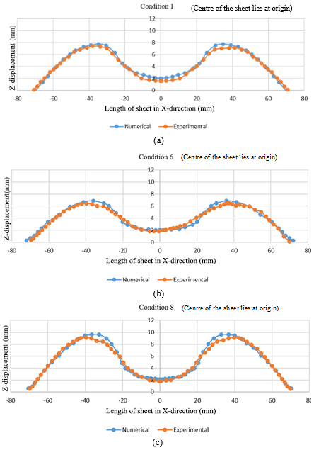
Figure 15 Numerical and experimental sheet height along the X direction. (a) Voltage = 2400 V, thickness = 1.02 mm, N=6. (b) Voltage = 2600 V, thickness = 1.63 mm, N=6. (c) Voltage = 2800 V, thickness = 1.22 mm, N=6.

5.5 Sheet deformation analysis

The sheet deformation was measured from experiments as well as from simulation. Experiments were performed as detailed in Table 2. The results at only three conditions are shown in Fig. 14 as an example. After deforming the profile of sheets was measured using a FARO Arm CMM machine (Anon, 2020). A complete profile was measured five times and average values were obtained. The experimental readings of sheet deformation were compared with numerical results, and only three conditions (i.e. conditions 1, 6 and 8) are presented in Fig. 15. From Fig. 15a to c it can be observed that numerical results are in close agreement with the experimental sheet deformation. The reason for error is attributed to the minimal variation in the coil and sheet gap during experimentation, which is a critical factor in defining magnetic pressure (Xiong et al., 2015).

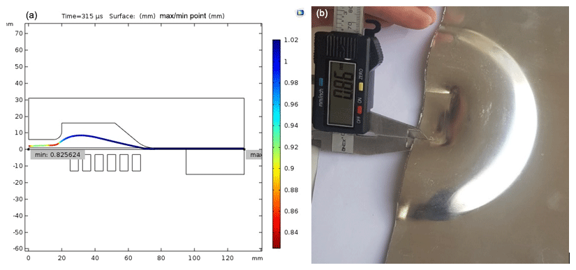
Figure 16 Minimum thickness of deformed sheet condition 1 (voltage = 2400 V, thickness = 1.02 mm, N=6). (a) Numerical result and (b) experimental measurement.

5.6 Sheet thickness analysis

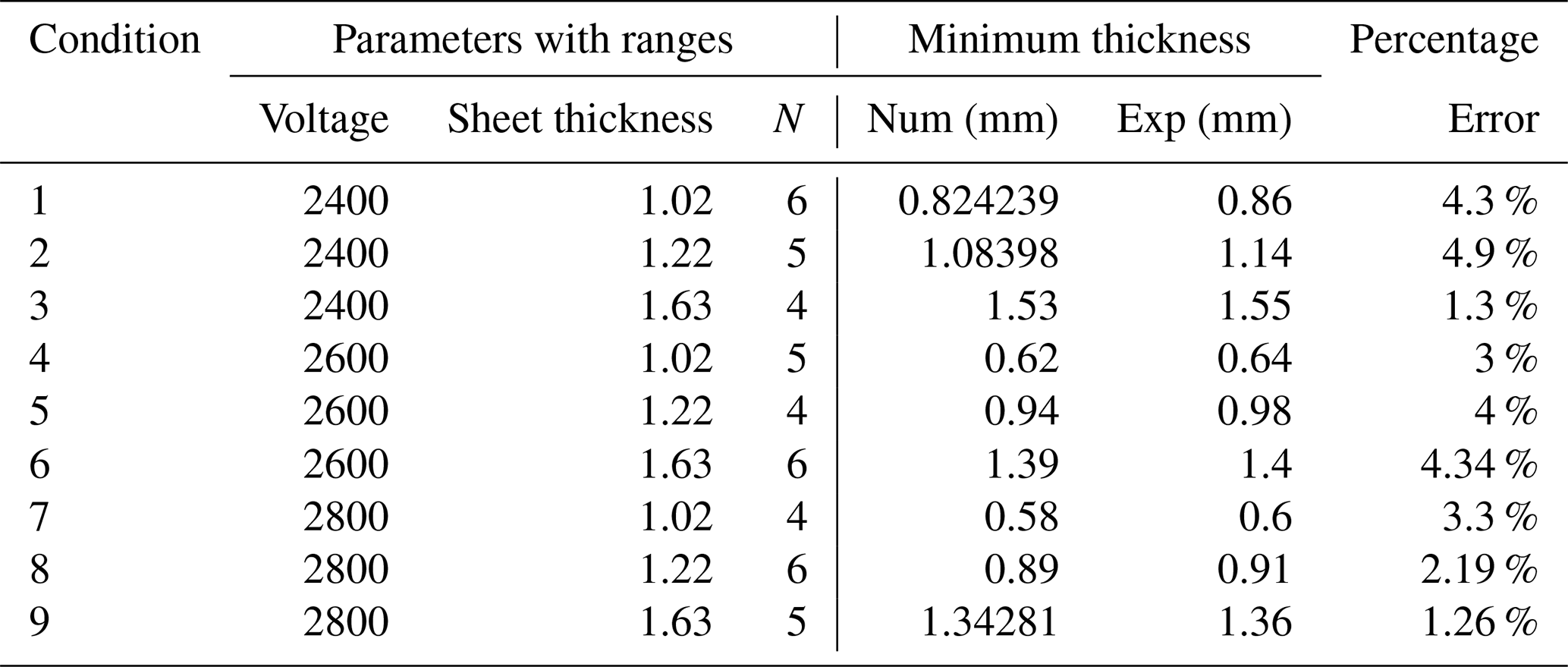
Sheet thickness for all conditions was obtained through simulation as well as experimentally by using a digital Vernier calliper as shown in Fig. 16. A total of five readings were taken at each point and the average value was tabulated in Table 4. For experimental condition 1, the minimum sheet thickness obtained was 0.824 mm, while the experimental sheet thickness was 0.86 mm (Fig. 16). The numerical and experimental values of minimum sheet thickness along with percentage error are mentioned in Table 4.

The phenomena of thickness reduction can be improved by making geometrical changes in the die. It can also be done by using lubrication or decreasing the blank holder force that can augment the deformation height, reduce the major strains and promote material flow and hereby improve sheet formability (Ma et al., 2018).

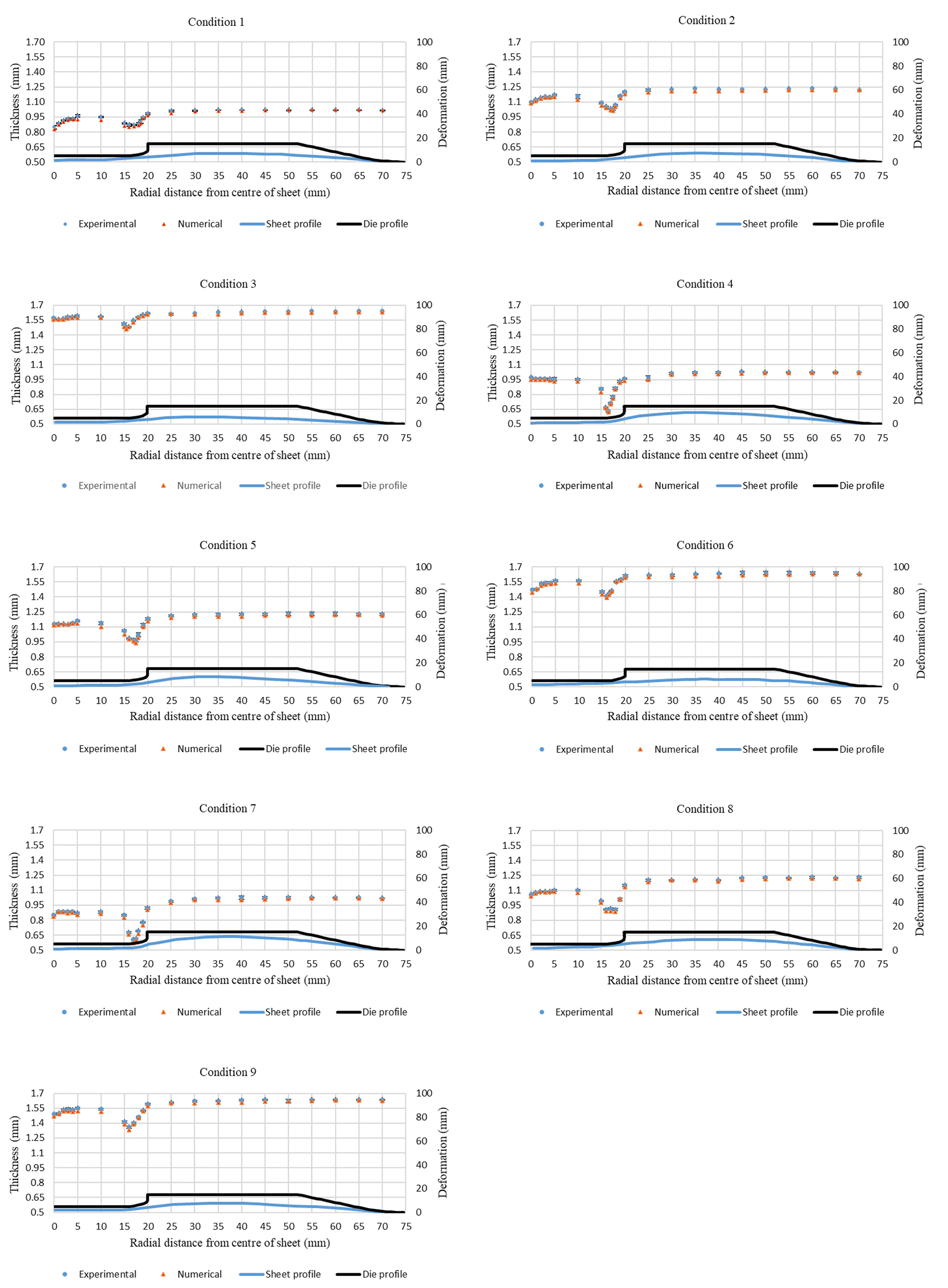
Figure 17 Numerical and experimental thickness of the sheet-on-sheet profile. (a) Voltage = 2400 V, thickness = 1.02 mm, N=6. (b) Voltage = 2400 V, thickness = 1.22 mm, N=5. (c) Voltage = 2400 V, thickness = 1.63 mm, N=4. (d) Voltage = 2600 V, thickness = 1.02 mm, N=5. (e) Voltage = 2600 V, thickness = 1.22 mm, N=4. (f) Voltage = 2600 V, thickness = 1.63 mm, N=6. (g) Voltage = 2800 V, thickness = 1.02 mm, N=4. (h) Voltage = 2800 V, thickness = 1.22 mm, N=6. (i) Voltage = 2800 V, thickness = 1.63 mm, N=5.

Table 5 Numerical and experimental sheet deformation.

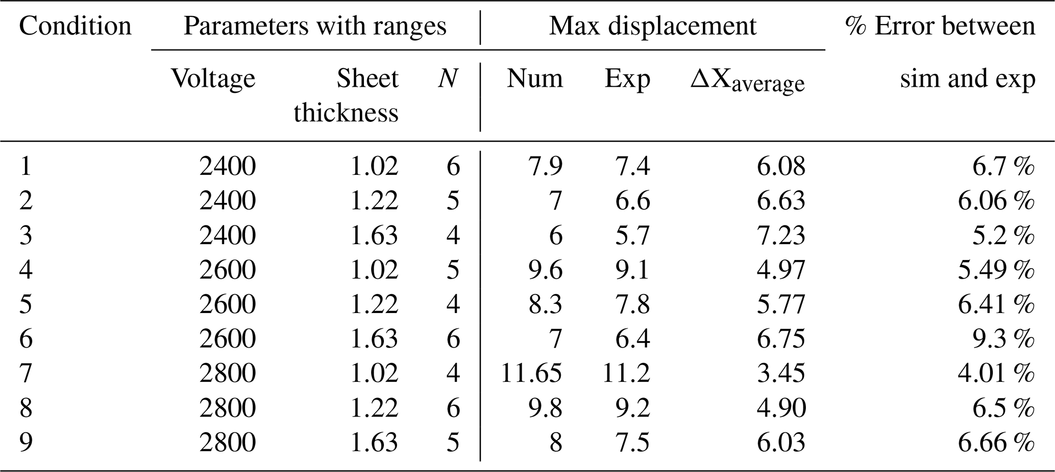
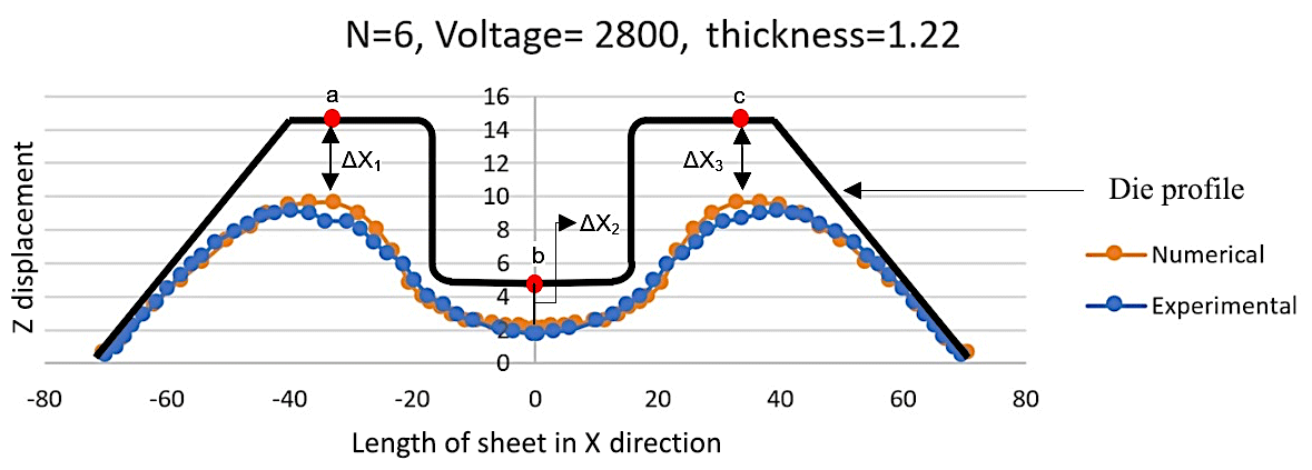
Figure 18 Difference between maximum values of point (a, b, c) for condition 8 (V = 2800 volts, thickness = 1.22 mm and N=6).

To analyse the thickness variation on the complete profile of the workpiece, the sheet profile was divided into 25 divisions starting from the centre of the die as shown in Fig. 17. The z displacement of the deformed sheet and the profile of the die are as per actual dimensions. The error bar chart shows the thickness variation of the sheet. The horizontal axis shows the radial distance from the centre of the sheet. The left-hand side vertical axis represents the sheet thickness variation at different points, both numerical and experimental values. The right-hand side vertical axis represents the sheet deformation and die profile.

Figure 19 Effect of processing parameters on ΔX_average.

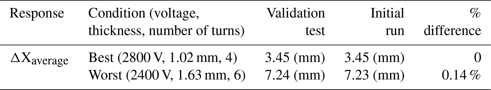
Table 6 Comparison of validation test results with initial runs.

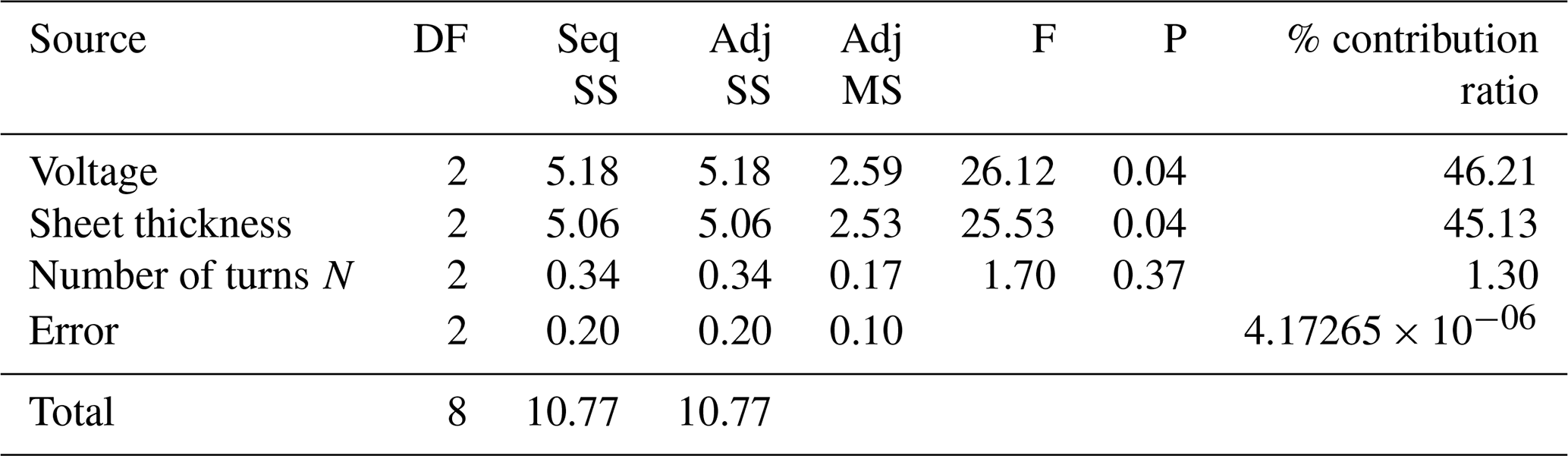
Two repeats of all the conditions in Table 5 were performed experimentally. The results were compiled and processed in MINITAB to perform analysis of variance (ANOVA). It can be seen from Table 7 that the applied voltage and sheet thickness are the significant process parameters. Applied voltage had the highest contribution of 46.21 %, followed by the sheet thickness with a contribution ratio of 45.13 %. The number of turns has the lowest contribution (1.3 %) towards sheet deformation. With increase in voltage, the induced current increases. This increased induced current results in higher Lorentz force and sheet deformation. Similarly, with increased thickness the deformation will reduce because of greater mechanical strength of thicker sheets. The number of turns effects the deformation as the inductance of coil increases with increasing number of turns, but that effect is very small compared to the effect of the other two parameters, which are voltage and sheet thickness. Error is just a description of the way the observations will vary from the means. In this case, the error is as small as $\mathrm{4.17}\times {\mathrm{10}}^{-\mathrm{6}}$.

Table 7 Analysis of variance of Z displacement for the three parameters used in this study.

From Fig. 17 it was observed that the experimental and numerical results were in good agreement for all nine conditions. It was observed that the two points where the thickness reduction mostly occurs are at the centre of the die, i.e. 0 and 15 mm distance. The reason for thickness reduction at 15 mm radial distance is the geometrical feature of the die. The thickness reduction at the centre of the die is mainly due to inertial forces: the centre point attains the highest velocity among all the other points, undergoing the highest deformation, as is evident from the velocity curve plot in Fig. 13. It was also observed that as the distance from the centre of the die increases, the reduction in thickness also decreases, which shows that the elongation in the sheet mostly starts from the centre of the sheet and reduces as it reaches the ends of the die. From the graphs, it can be observed that with increasing voltage, the thickness reduction at the centre and intricate geometries will enhance due to an increase in the velocity of the sheet and collision of the sheet with the die profile. By increasing the number of turns in the coil, the peak velocity of the sheet is reduced, which results in less thickness reduction. For thicker sheets, the velocity of the sheet will decrease and will result in less reduction in thickness.

6 Statistical analysis of sheet deformation

The average gap between the die profile and deformed sheet height was obtained at three points a, b and c as shown in Fig. 18. ΔX₁, ΔX₂ and ΔX₃ represent the gap between the die and deformed sheet at points a, b and c respectively. ΔX_average shows the average of ΔX₁, ΔX₂ and ΔX₃. A smaller value of ΔX_average means better sheet deformation and vice versa.

The main effect plot was used to find out the best and worst conditions for sheet deformation. From Fig. 19 the ΔX_average reduces with increasing voltage but increases with increasing sheet thickness and number of turns of the coil. With increase in voltage the magnitude of Lorentz forces between the sheet and coil increases, which results in greater deformation in the sheet. The increased thickness means the workpiece is heavier and has greater mechanical strength, which results in a larger value of ΔX_average (Dordizadeh et al., 2011). As turn count increases, the coil inductance increases. Therefore, the coil turn count (i.e. inductance) is optimized at a value such that large magnetic fields are created while still allowing large currents (Thibaudeau and Kinsey, 2015).

The minimum value of ΔX_average is at condition 7, while the maximum is at condition 3.

6.1 Validation experiments

The validation experimentation of the best and worst conditions for ΔX_average was performed (Table 6). The results revealed that minimum and maximum ΔX_average were 3.45 and 7.24 mm at the best and worst conditions respectively, which were in good agreement.

7 Conclusions

A fully coupled FE model was developed to analyse the behaviour of a workpiece in the electromagnetic forming process. The effects of voltage, sheet thickness and the number of coil turns on Lorentz force, velocity profile, sheet deformation and sheet thickness variation were analysed. Taguchi design of experiments was used to analyse and compare experimental sheet deformation and thickness variation with numerical results. Statistical analysis and ANOVA were carried out to identify significant parameters and their contribution.

From the FE simulations, it was revealed that the magnetic flux reached its highest value of 3.68 T at 100 µs. The flux was found to be related to the current that passes through the coil. By keeping the other process parameters constant, increasing the sheet thickness reduces the Lorentz force due to changes in the distribution of the induced current. In the simulation, generally for all parameters, the sheet deforms due to magnetic force for the first 100 µs of the cycle time, while after 100 µs the deformation is associated with the inertial force. Spring back phenomenon was observed in the closed die configuration. This spring back is associated with the reduction in the maximum deformation and may also cause wrinkling and tear. The velocity of the sheet varies at different points across the profile of the sheet. Point C moves first due to high magnetic force during the first 100 µs time step. Points “B” and “A” start moving after 100 µs. The motion of “A” and “B” is due to a combination of magnetic and inertial forces exerted by initial movement of point C. An unstable zone of the velocity profile showed the random movement of the sheet after hitting the die profile. This deformation in the unstable region is attributed to inertia forces.

Numerical simulation and experimental results of sheet thickness at various points along the profile of the final part were in good agreement. The maximum percentage error was observed to be 4.9 %, corresponding to condition 2 (voltage of 2400 V, sheet thickness of 1.22 and number of turns of the coil as 5). The thickness reduction takes place at the centre block and at the edges of the centre block where there is sharp change in the profile of the die, which indicates maximum plastic deformation in these regions.

Statistical analysis of the experimental results showed that the applied voltage and sheet thickness are significant parameters for sheet deformation, whereas the effect of the number of turns of the coil was found to be insignificant. The contribution ratio of voltage was 46.21 % and that of sheet thickness was 45.13 %.

Appendix A: Abbreviations and nomenclature

σe	Electrical conductivity
ANOVA	Analysis of variance
PTR	Percentage thickness reduction
ΔXaverage	Difference between sheet and die profile
N	Number of coil turns
MF	Magnetic field
SM	Solid mechanics
s	Sectional area of the coil
ω	Angular frequency
R	System resistance
B	Magnetic flux density
β	Damping coefficient
E	Electric intensity
H	Magnetic intensity
J	Current density
L	System inductance
M	Mutual inductance
δ	Skin depth