the Creative Commons Attribution 4.0 License.
the Creative Commons Attribution 4.0 License.
 | 31 Jul 2020
Design and Robustness Analysis of Intelligent Controllers for Commercial Greenhouse
Mattara Chalill Subin
Abhilasha Singh
Venkatesan Kalaichelvi
Ramanujam Karthikeyan
Chinnapalaniandi Periasamy
In a commercial greenhouse, variables, such as temperature and humidity, should be controlled with minimal human intervention. A systematically designed climate control system can enhance the yield of commercial greenhouses. This study aims to formulate a nonlinear multivariable transfer function model of the greenhouse model using thermodynamic laws by taking into account the variables that affect the Greenhouse Climate Control System. To control its parameters, Mamdani model-based Fuzzy PID is designed which is compared with the performance of proportional-integral (PI) and proportional-integral-derivative (PID) controllers to achieve a smooth control action. The Fuzzy logic based PID provides robust control actions eliminating the need for conventional tuning methods. The robustness analysis is performed using values obtained from real-time implementation for the greenhouse model for Fuzzy based PID, PI and PID controllers by minimizing the Integral Absolute Error (IAE) and Integral Square Error (ISE). The greenhouse model has strong interactions between its parameters, which are removed by Relative Gain Array (RGA) analysis, thereby providing an effective control strategy for complex greenhouse production. Further, the stability analysis of non-linear greenhouse model is conducted with the help of the bode plot and Nyquist plot. Results show that good control performance can be achieved by tuning the gain parameters of controllers via step responses such as small overshoot, fast settling time, less rise time, and steady-state error. Also, smoother control action was obtained with Fuzzy based PID making the Greenhouse Climate Control System stable.
- Article
(3702 KB) - Full-text XML
- BibTeX
- EndNote


Climate control system (CMS) is an important component for the automation of the commercial greenhouses comprising control modules interfaced with a central control system. Bluetooth devices can be integrated with CMS systems, which share the information in a faster manner using piconets. In a piconet system, one Bluetooth device will act as a master and the remaining devices will act as slaves. Piconet allows a maximum of seven slaves in a system with a master device (Olenewa, 2013). The configuration between two Bluetooth devices is wireless, which makes the system interconnection easy. The piconet Bluetooth networks are user-specific and restrict other networks in the system, thereby making it highly reasonable for multi-span commercial greenhouses. Bluetooth technology in agricultural automation is one of the revolutionary approaches in greenhouse automation that has attracted considerable research interest. Kim et al. (2006) developed an irrigation system interfacing the information of soil and water system with the development of a sensor interface with a Bluetooth device. The feedback loop is connected to a system of linear sprinklers controlled by a programmable logic controller (PLC) which processes the feedback information from the base system and controls the water irrigation parameters thereby controlling the water requirements for plant growth. In open field cultivation, plants require sunlight, soil, and water for crop production (Saha et al., 2016). Controlling the temperature is one of the important aspects in yield management of agronomy. Besides, maintaining water as well as moisture content is another imperative factor in indoor cultivations in a controlled water environment by preventing wastage (Bilderback et al., 1999). Among various irrigation technologies, drip irrigation has been proven as the most effective technology owing to its conservation measures (Alderfasi and Nielsen, 2001). Furthermore, it can control the water level required for plant growth.
Water supply to plants in an agronomical industry is being controlled using various techniques. Conventionally, farmers used to control this by routine inspections at various intervals in a day. Further advancement occurred with the innovations using timers, which can switch drip irrigation mechanisms on and off to control the agro-water distribution (Akkuzu et al., 2013). Advancement in agronomy led to the development of Crop Water Stress Index (CWSI) (Alderfasi and Nielsen, 2001; Akkuzu et al., 2013), which controls water level required to schedule the irrigation demand (Irmak et al., 2000; Teitel, 2007). CWSI helps farmers to determine the best combination for the soil moisture content in conjunction with the yield management for the vaporization (Kittas et al., 2005). Calibration curves obtained can help to identify the crop variety that can enhance the measurement accuracy of the parameters that are influencing the yield management. Indoor environment control is one of the important factors that drive commercial greenhouse production. Important elements driving the indoor environment include temperature, relative humidity, air velocity, and radiation emissions (Marucci and Cappuccini, 2016). Major control tools that can regulate the above parameters are shade curtains, fans, and air vents. Indoor environment factors and the control factors are highly interconnected with network CMSs (Akkuzu et al., 2013). Therefore, the development of intelligent CMSs with the help of sensors as field devices will facilitate real-time output control (Puglisi et al., 2017). The optimum output is the wherewithal of improved crop production inside the greenhouse (Adeyemi et al., 2018; Pucheta et al., 2006; Hu et al., 2011b). The proposed study emphasizes commercial greenhouse Climate Control System to integrate the field sensors with control tools and drip irrigation systems for controlling the indoor environment. Power supply for the commercial greenhouses is an important factor which will drive the investment due to its high transmission cost, this can be sorted out by using the hybrid renewable energy systems using the photovoltaic (PV) panels and wind turbines (WT), this has been tested and found acceptable using adaptive inertia based particle optimization (PSO) (Alireza and dos Santos Coelho, 2015). To reduce the operational cost of the commercial greenhouse, the reduction in energy consumption from the HVAC system will make an important contribution and this can be achieved by daily optimal chiller loading optimization (DOCL) (dos Santos Coelho and Alireza, 2016). A wavenet (Trierweiler Ribeiro et al., 2019) enabled future load forecasting from data can also help to improve the efficiency of the commercial greenhouse to have better energy management. Non-linear model predictive control (NMPC) (Faccini Santoro et al., 2019) approach can study the effectiveness of energy management approach in HVAC systems without compromising the indoor thermal comfort by providing a balance between temperature and relative humidity in the commercial greenhouses. Hygroscopic characteristic of the building corners (dos Santos Coelho and Alireza, 2016) will impact the energy consumption of the commercial greenhouses.
Commercial Greenhouse Control system has to monitor and control temperature, humidity, pH, carbon dioxide CO2 and fogging. Meihui et al. (2017) proposed greenhouse climate control using decoupling technique to separate CO2 concentration, temperature and humidity and PID controller is designed to track the setpoints whereas in Faouzi et al. (2017) proposed fuzzy-based self-tuning of PID controllers to control temperature and humidity but this study lags stability and robustness analysis. Chaudhary et al. (2019) proposed observer-based PID controller to control the indoor variables like inlet temperature and humidity and author has used Fuzzy rule base for the enrichment of CO2. In this study, there is no stability analysis carried out. Susanto et al. (2018) discussed the design of PLC based control system with PID controllers for rotary fixture and stability analysis was carried out using Routh-Herwitz criteria and Nyquist plot. Premkumara and Manikandan (2018) discussed the stability and robustness analysis of ANFIS tuned PID controller for brushless DC motor. The author carried out the robustness analysis of controller by varying the inertia, flux and resistance of motor from 50 % to 200 % and also stability analysis was carried out using Nyquist plot.
Based on the extensive literature analysis, this paper concentrates on the modelling and control of a fully autonomous commercial greenhouse with the implementation of fuzzy PID and PID controllers to control the inlet temperature and relative humidity. The main objective is to reduce the error in inlet temperature and humidity thereby reducing the minimal use of energy consumption. Using MATLAB/Simulink models, fuzzy PID controller for humidity and temperature are designed and its performance is compared with the PID controller along with the disturbances namely solar radiation, outlet temperature and humidity. Stability analysis is also performed using Bode plot and Nyquist plot for greenhouse. Also, Robustness analysis for both controllers is analysed under 2 % and 15 % variations which are decided based on operating regions obtained from the open-loop analysis of greenhouse. Further the simulation analysis has been verified with experimental results. The proposed decoupling method using RGA analysis method can be effectively used in the greenhouse for temperature and humidity control in the countries like the United Arab Emirates where cooling is a major concern.
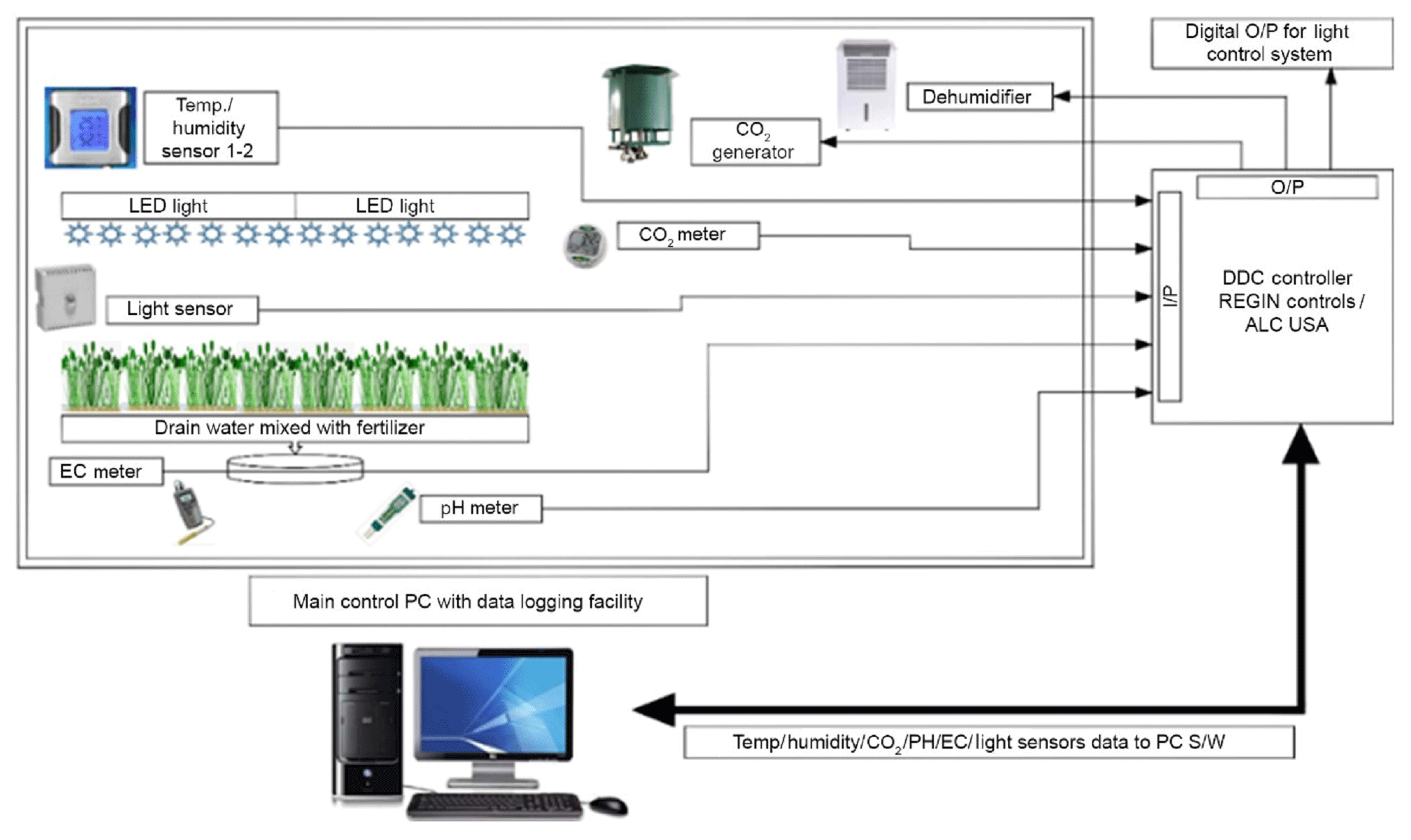
Climate control module with a central control which is interfaced with all the field devices has been tested in a real-time scenario.
During the night, plants will consume more CO2, manure, thereby providing adequate irrigation supply. Another important factor affecting the plant growth during the day is the variation in indoor variables like temperature and humidity due to the disturbances from external conditions. Systematically designed Climate CMS can enhance the yield of the commercial greenhouses, resulting in healthier crop production. Test locations have been established in different regions of the greenhouse. All the field test locations are shown in Fig. 1. During the O position, all the central sensing station will be active and sense the logging information at a rate of 11 000–11 600 bits per second (bps). LICOR temperature/quantum sensors (LI 190S) and humidity sensors (LI 7200), which can automatically log the data are used to log the data from the specified locations. In locations, 1–6 of the greenhouse, central loggers are used to record the data into a source file. CMS module has been developed with a communication distance from 80 to 120 m with a 20 dBm output transmittance at a maximum frequency of 2500 MHz. However, the central CMS station host unit and transmitting field devices need to be carefully placed without any obstruction in between, which may affect the communication. The experiment was conducted in the Al Khawaneej District, Emirate of Dubai, United Arab Emirates. The test was conducted in the climate control module with a microcontroller as a sensing unit for validation and evaluation of its efficiency in transmitting data. The upgraded controller has been tested for the real control operation of one of the greenhouses for a small production cycle (18 d) and the fluctuations in temperature and humidity obtained were within the permissible limits.
3.1 Multivariable Greenhouse
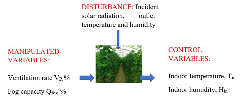
Generally, a mathematical model is a simplified representation of any system. The mathematical methods and complexity in solving these models require good control knowledge. This work analyzes the dynamic system of commercial greenhouse environment. In the literature available, greenhouse dynamics modeling and different control strategies have been reported. The models related to the horticultural industry often require considerable extra programming effort to render them sufficiently user friendly. The model described herein is a highly nonlinear model intended for scientific research.Two popular approaches for greenhouse modeling include energy and massflow based approach and experimental data based approach (Hu et al., 2011b). This paper deals with energy balance approach proposed by Pasgianos et al. (2003). The analytical modelling and controls based on the state-space form is shown in Eq. (1).
where x represents state variables; herein, state variables are inlet temperature Tin (∘C) and inlet humidity Hin (g m−3); u are the manipulated inputs, such as fog capacity Qfog (%) and ventilation rate VR (%); v is external disturbances like solar radiation energy Si, outdoor temperature Tout, and outdoor humidity Hout; t denotes time, and f(.) is a nonlinear function. To effectively validate the stability analysis, state-space is converted into the transfer function model. The functional block diagram of the greenhouse model is provided in Fig. 2.
3.2 Dynamic Modeling of Greenhouse Climate Model
To simplify the model and reduce the complexity of computation, the work is focused on only primary disturbance variables. After normalizing the controlled variables, the governing equations for the dynamic model of the greenhouse are presented using the following differential equations Eqs. (2) and (3) (Hu et al., 2011b; Pasgianos et al., 2003).
where Tin∕Tout is the indoor/outdoor air temperature (∘C), Hin∕Hout is the indoor and outdoor humidity ratios; (g [H2O] kg−1 [dry air]), UA is the heat transfer coefficient of the enclosure (W K−1), Co=ρCpVth, where ρ and Cp are air density and specific heat of air, respectively, Vth is 60 %–70 % of the geometric volume of the greenhouse, Si = solar radiant energy (W), , where λ is the latent heat of vaporization (J g−1), and is maximum water capacity of fog system, , where α is constant scaling parameter, , and tv is the time needed for one air change.
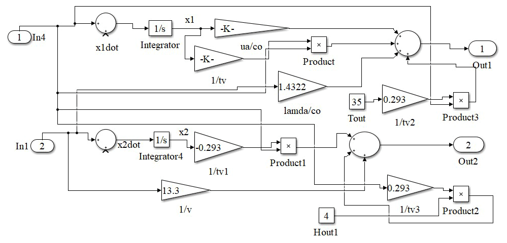
The open-loop analysis using Eqs. (2) and (3) deals with the combined response of the greenhouse model with different initial conditions excluding the effect of the feedback loop. Greenhouses are highly nonlinear; therefore, to obtain the linearized transfer function model, an attempt has been made to implement an open-loop analysis with step input change. The manipulated variables (inputs) namely ventilation rate VR,% and water capacity of the fog system Q%,fog is applied to the open-loop model and corresponding outputs inlet temperature Tin and inlet humidity Hin are obtained. It is found that the open-loop response deviates from the reference value, which is termed as an error or offset. The dynamic model of the greenhouse using the above equations is shown below in Fig. 3. The above steps can be accomplished using a system identification toolbox in MATLAB using the command “ident” in the command window. The block diagram of the modeling part that has been executed for the greenhouse is given below in Fig. 4.

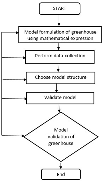
3.3 System Identification for Greenhouse Model
The key idea behind system identification is investigating the behaviour of a model structure by recording the input-output using continuous or discrete-time signals. The system herein is assumed to be a black box to the user. The basics steps involved in system identification as mentioned in Ljung (1987) are as follows:
-
Step 1: Collection of data from a mathematical model by applying step response.
-
Step 2: Choosing the model from trial and error.
-
Step 3: Selection of the best model that fits the process from available models. Herein, VR,% and Q%,fog of the greenhouse are applied to system identification toolbox and corresponding Tin and Hin are recorded. Based on the best fit value the process transfer function model of the greenhouse is obtained.
-
Step 4: From this process model, a controller for the greenhouse is designed. The simplified flowchart for system identification is given below in Fig. 5.
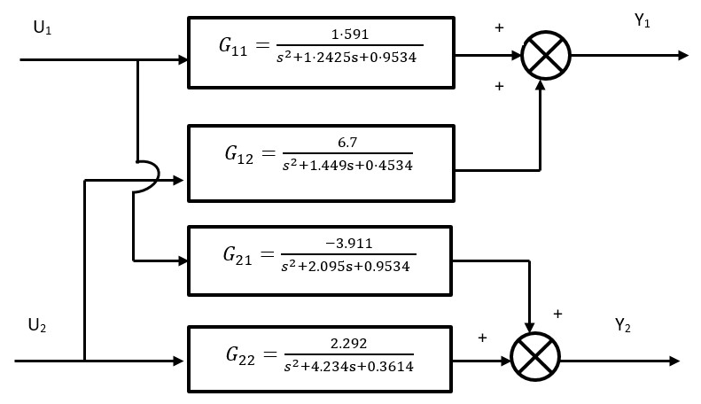
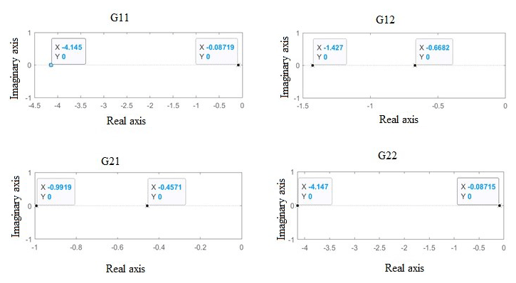
The transfer functions of greenhouse obtained from system identification are given in below equations Eqs. (4) to (7).
From the above equations, G11 transfer function relates inlet temperature and ventilation rate, keeping the fog capacity constant; G12 relates inlet temperature and fog capacity, keeping ventilation rate as constant; G21 relates inlet humidity and ventilation rate, keeping fog capacity as constant; and G22 relates inlet humidity and fog capacity, keeping ventilation rate as constant. The block diagram representing multiple input multiple output (MIMO) of a greenhouse model using the above transfer functions in MATLAB/SIMULINK is shown below in Fig. 6.
4.1 Description of Control Model for Greenhouse
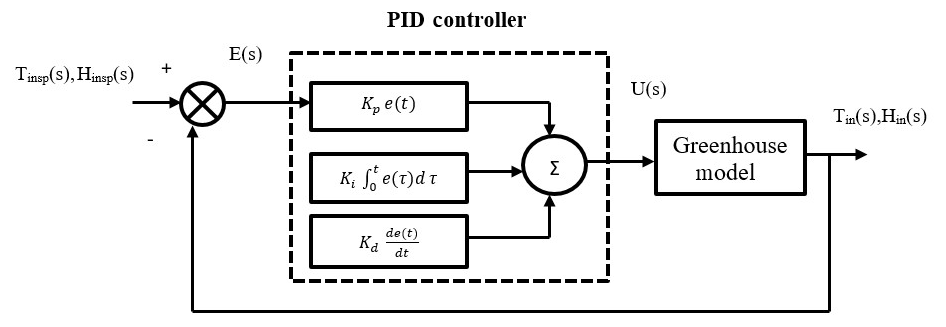
PID controllers have a wide range of applications for industrial process control. The proportional term produces an output proportional to the error and these controllers require bias and provide a stable operation with offset (steady-state error). To remove the steady-state error, the integral term is introduced and in most of the industrial applications, the PI controller is preferred because the high-speed response is not required. To anticipate the future behaviour of the plant, a derivative term is used where the output is proportional to the rate of change of error. The general mathematical description of PID mentioned in Chang (2007), Arruda et al. (2008) is generally written in the ideal form in Eq. (8).
where Kp = proportional gain, Ti = integral time, Td = derivative time, is the integral gain, Kd=KpTd is the derivative gain, and e(t) is the current error signal as described in Eq. (9).
where x(t) is the controlled variable of a plant (output), which includes the inlet temperature Tin and inlet humidity Hin and u(t) is manipulated variable, which includes ventilation rate and water capacity of fog system of greenhouse respectively. The general block diagram of the PID controller for the greenhouse is shown below in Fig. 7.
4.2 Design of PID Controller for Greenhouse
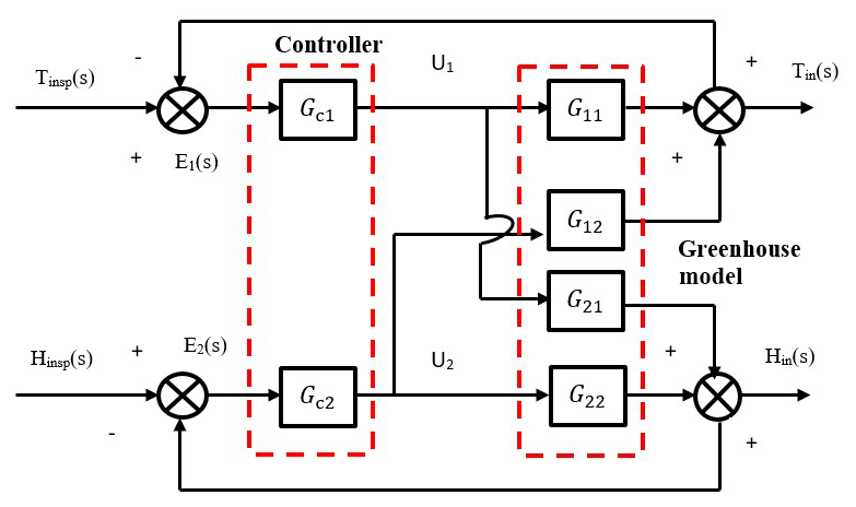
The greenhouse dynamic model mentioned in this work is a multivariable nonlinear system (Pohlheim et al., 2000; Killingsworth and Krstic, 2006). In CMS aspects, if there are multiple inputs and outputs for a particular system, there is a requirement to design many controllers, which is practically impossible and not cost-effective. Therefore, to optimally decide the number of controllers based on input-output relationship, relative gain array (RGA) analysis is conducted. RGA analysis was proposed by Bequette (2010) and is a powerful tool for the input-output pairing of linear multivariable plants. An appropriate choice of input-output pairs before the commencement of the controller design is vital for optimal closed-loop behaviour. The RGA analysis involves formation of gain matrix from transfer function Gp(s) which determines the influence of each input variable with the output. This analysis will be useful for decoupling the variables which makes controller design much easier (Pohlheim et al., 2000). A ratio of this open-loop gain to this closed-loop gain is determined and the results are displayed in a matrix. Transfer function matrix Gp(s) for a greenhouse model is given below in Eq. (10).
The RGA matrix is calculated by substituting s=0 in Eq. (10) and the values are given below in Eq. (11)
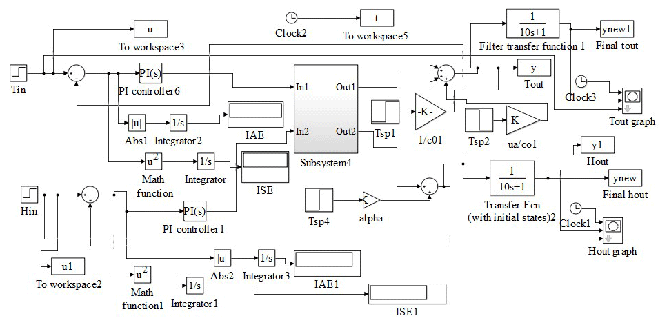
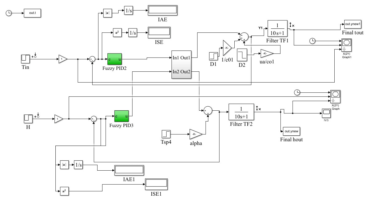
According to Bequette (2010), the recommended pairing for the controller are matrix elements, which corresponds to negative pairings, should not be selected and the value that is closer to 1 is chosen. It is observed from the above RGA matrix K that optimal pairing is Y1–U1 an Y2–U2. The general block diagram for the multiloop greenhouse model is mentioned in Fig. 8. The MATLAB/SIMULINK diagram for greenhouse model with PID and PI controller is shown below in Figs. 9 and 10.
4.3 Design of Fuzzy based PID Controller for Greenhouse
In fuzzy logic control, the process is controlled by the formation of rules based on the human expert knowledge which are called as fuzzy rules or relations (Chaudhary et al., 2019). Hence fuzzy logic controllers may be reflected as nonlinear PID controllers whose parameters can be resolute based on the error signal and their time derivative or difference (Zanetti Freire et al., 2016). In this paper, fuzzy logic PID is used to create a rule base for gain scheduling of controller parameters Kp and Kd is proposed for greenhouse control (Zhao et al., 1993). It is demonstrated in this paper that better robust and stable control performance can be expected in the proposed method than that of the conventional PID controllers. The following are the steps involved in designing the Fuzzy Logic PID controller is shown in Fig. 11.
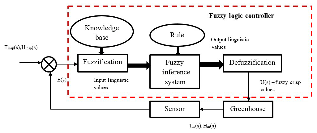
4.3.1 Step 1: Identification of Variables
There are two input variables needed for greenhouse model namely e(k) and Δe(k) and three output variables taken for analysis namely Kpp, Kdp and alpha.
4.3.2 Step 2: Determination of Fuzzy Sets
The inputs and outputs are associated with membership functions forming a fuzzy set and each fuzzy sets have linguistic labels. In this proposed work input fuzzy sets are NB-Negative Big, NM-Negative Medium, NS-Negative Small, ZO-zero,PB-Positive Big, PM- Positive Medium, PS- Positive Small. Small and Big are considered as output fuzzy sets.
4.3.3 Step 3: Generation of the Membership Function
Membership function quantifies the linguistic labels and represents the fuzzy sets graphically. A membership function for a fuzzy set A on the universe of discourse X is defined as where the degree of membership varies between 0 to 1. The membership function used for input variables are trapmf,trimf whereas for output variables Kpp and Kdp, guassmf is used and for alpha,trimf singleton membership function is used. The membership functions are illustrated graphically and is shown in Fig. 12a–e.
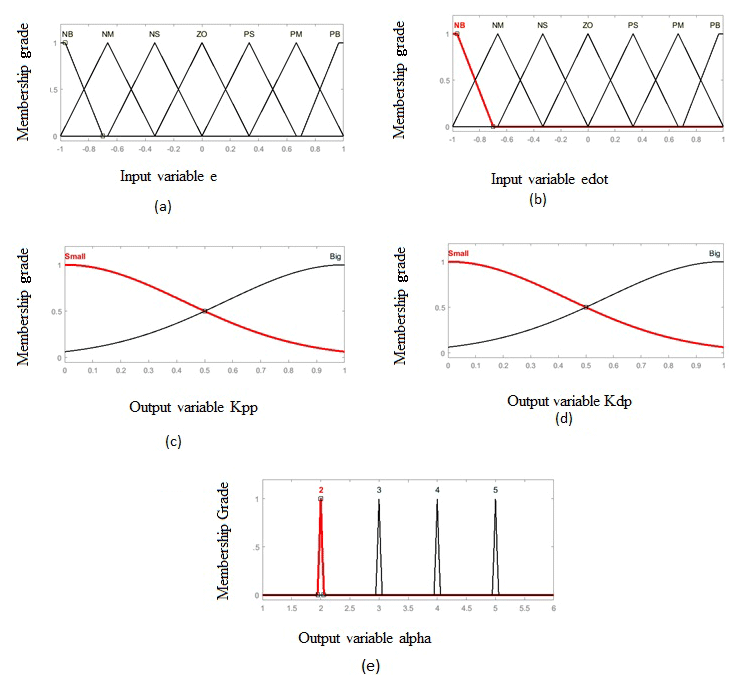
Figure 12(a) Membership Functions for Input Variable e, (b) Membership Functions for Input Variable edot, (c) Membership Functions for Output Variable Kpp, (d) Membership Functions for Output Variable Kdp and (e) Membership Functions for Output Variable alpha.
4.3.4 Step 4: Formation of Fuzzy Rule Base
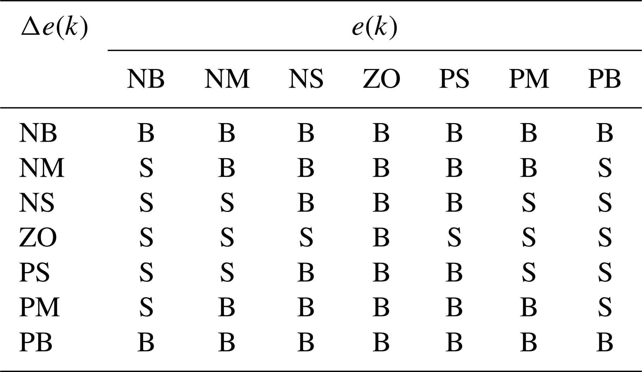
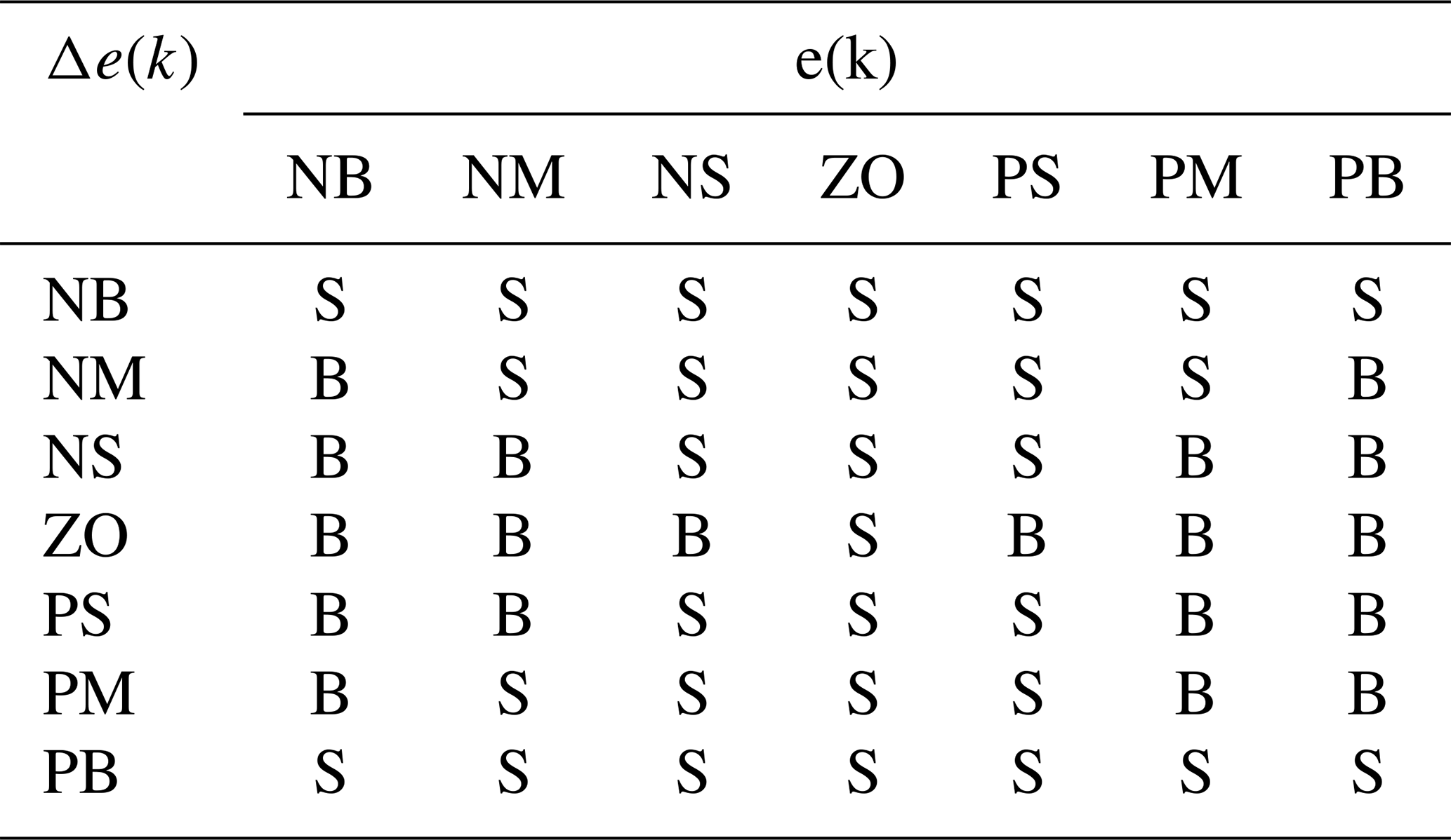
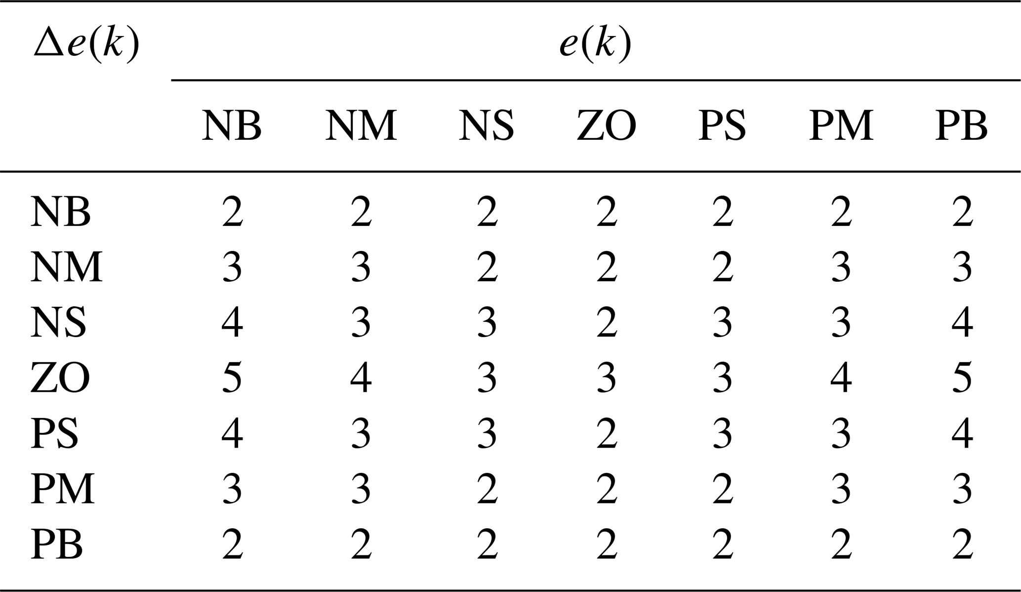
Rule base defines the input-output relations and stores the knowledge of the entire process so that the inference engine can use this rule base to obtain the output fuzzy linguistic variables. In this work, 49 tuning rules for Kpp, Kdp and alpha have been formulated for fuzzy-based PID which are mentioned in Tables 1, 2 and 3 respectively. The rules are stored in IF-THEN format or IF-THEN-ELSE format.
4.3.5 Step 5: Fuzzification
In this step, crisp input variables are transformed into fuzzy sets with the help of membership functions.
4.3.6 Step 6: Fuzzy Inference System
Fuzzy inference engine evaluates the IF-THEN rule base and combines results obtained from each rule. For example, rules are formulated as below,
IF e(k) is NB AND Δe(k) is NB THEN Kpp is big, Kdp is small AND alpha = 2.
4.3.7 Step 7: Defuzzification
This step finally converts fuzzy sets obtained from the inference system into crisp output values Kpp, Kdp and alpha. Based on the obtained values, PID controller is tuned to perform necessary control action. The tuning values are calculated by using equations Eqs. (12) to (14) and min and max values are mentioned in Table 5.
Where, Kp = Proportional gain, Kd = Derivative gain and Ki= Integral gain.
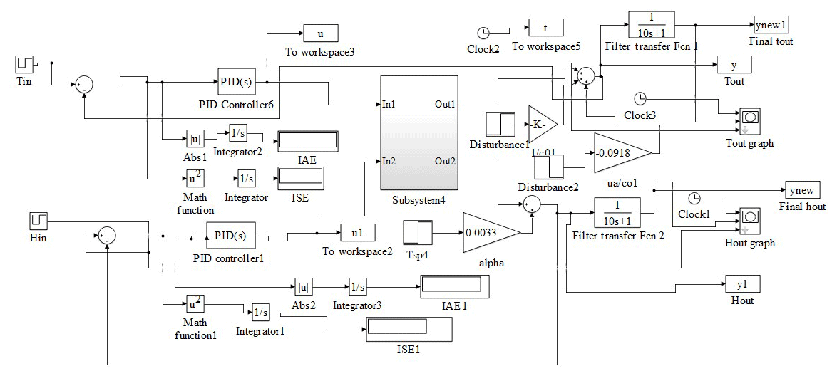
The MATLAB/SIMULINK diagram for greenhouse model with Fuzzy based PID controller is shown below in Fig. 13.
4.4 Comparative Studies on Intelligent Controllers with Conventional Controllers for Greenhouse System
In this section, simulation results of the proposed real-time greenhouse model with the intelligent controller like Fuzzy Based PID is implemented and also comparative results using PID controllers are presented. The identified parameters of the greenhouse are specified, as shown in Table 4 (Hu et al., 2011a, b). For this analysis, surface area and height of greenhouse is considered as 1000 m2 and 4 m, respectively. The solar radiation is reduced to 60 % by using special covering material which is 300 W m−2 (Hu et al., 2011b; Pasgianos et al., 2003). The maximum water capacity of fog system varies from 1.3 to 26 g [H2O] min−1 m−3. The maximum ventilation rate is chosen as 20 air changes per hour, which is converted into a step change of 13–19.99 m s−1.
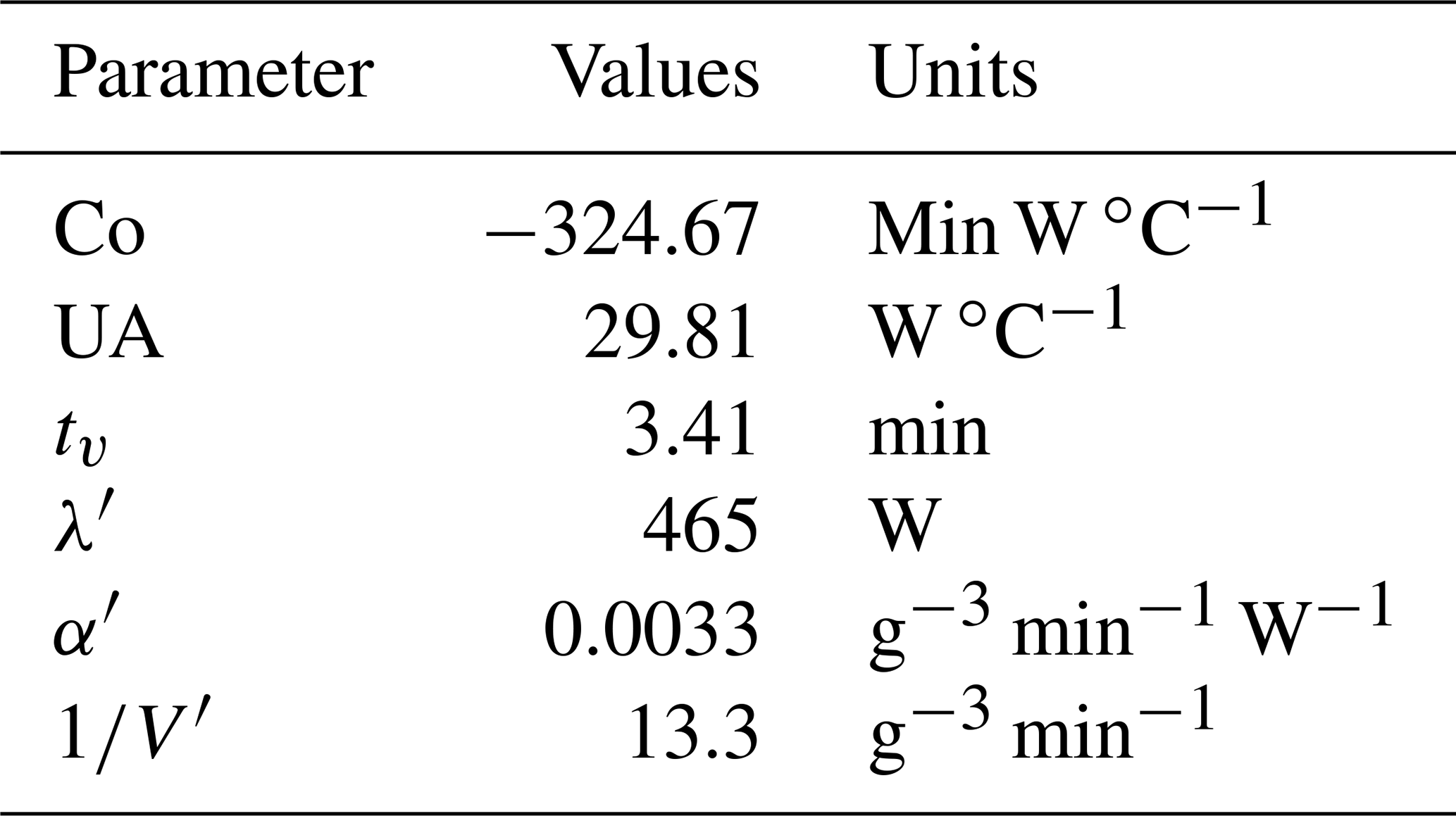
Table 5Tuning parameters of conventional controllers for greenhouse.
The active air mixing volume of temperature and humidity are specified (Hu et al., 2011a, b) as Vth=0.65 V. With respect to RGA analysis, as discussed in Sect. 2. the setpoint tracking test for controller outputs for inlet temperature and relative humidity, respectively, is illustrated. The setpoint changes of inlet temperature and humidity ratios are varied between increasing and decreasing steps ranging from 18 to 21 ∘C (Tin) and from 16.5 to 19.5 g [H2O] kg−1 (Hin). The output is obtained for every sample time of 400 s, and in every setpoint change, there exists a steady-state error. After applying tuning parameters as shown in Table 5 for the greenhouse model using PI and PID controller, a smooth closed response is observed, and steady-state error is removed.
It is observed from Fig. 14a and b that because of integral action peak overshoot, which is nothing but maximum peak value of output with respect to the input signal is approximately 15.6 % and there is no peak overshoot in the inlet humidity. Also, it takes 93 samples and 250 samples to reach steady state for inlet temperature and inlet humidity respectively. A PID controller was designed and implemented through simulation as shown in Fig. 15a and b. It is observed that there is the only an initial peak value of 24.8 in temperature and humidity which is considerably less than 30 with PI controller and inconsequent samples smoother response is obtained. Also, the controller utilizes only 60 and 50 samples to achieve steady-state in inlet temperature and humidity. It is assumed that by keeping the disturbance variables as constant, for every 400 samples, a setpoint change in temperature and humidity is produced, and it is observed that there is no steady-state error and overshoot.
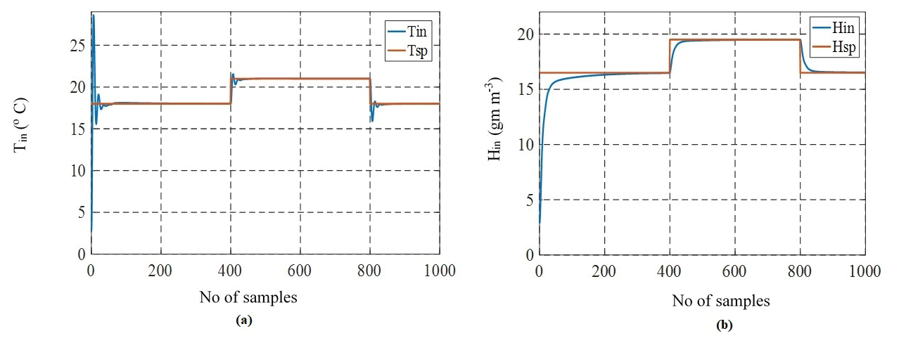
Figure 14(a) Closed-Loop Response of Inlet Temperature Tin for Step Changes in Temperature with PI Controller and (b) Closed-Loop Response of Inlet Humidity Hin for Step Changes in Humidity with PI Controller.
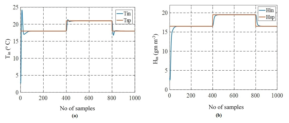
Figure 15(a) Closed-Loop Response of Inlet Temperature Tin for Step Changes in Temperature with PID Controller and (b) Closed-Loop Response of Inlet Humidity Hin for Step Changes in Humidity with PID Controller.
The Fuzzy based gain scheduling of PID gains for the greenhouse is implemented to control the inlet temperature and inlet humidity and Fig. 16 shows the Mamdani model of fuzzy-based inference system implemented in MATLAB. It is observed from the Fig. 17a and b that there is no initial overshoot with Fuzzy PID and smooth control action is achieved for step time of every 400 s with faster settling time of 1.13 and 1.72 samples whereas PID controller took 60 samples to reach steady state. Also with fuzzy PID error values in temperature and humidity obtained are lower than conventional PID controller. Here disturbance variables are kept constant and setpoint change is analyzed for every 400 samples for a total time of 1000 samples.
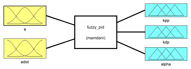
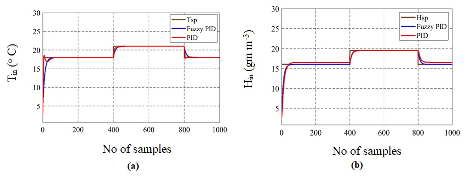
Figure 17(a) Comparative Analysis of Step Changes in Inlet Temperature Tin with Fuzzy PID and PID Controller and (b) Comparative Analysis of Step Changes in Inlet Humidity Hin with Fuzzy PID and PID Controller.
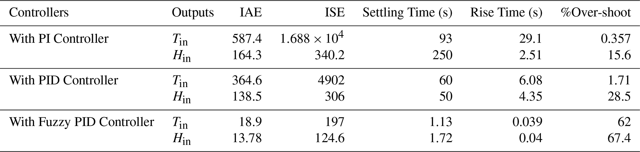
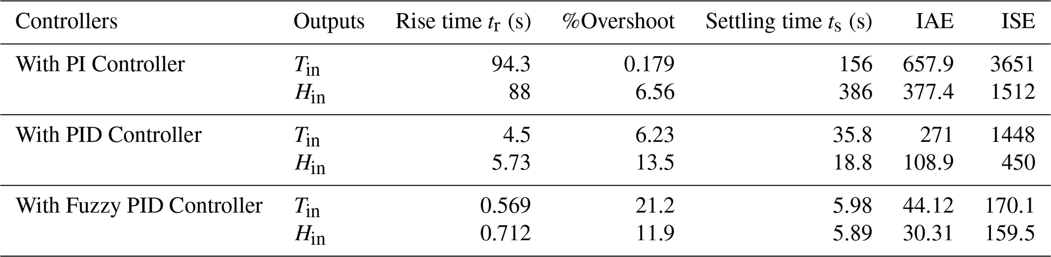
Table 6 depicts a comparative study of performance characteristics of the greenhouse model designed with PI, PID and Fuzzy based PID controllers. It is inferred that Integral Absolute Error (IAE) and Integral Square Error (ISE) are less with Fuzzy based PID controller with the value of 18.9 and 197 for inlet temperature and 13.78 and 124.6 for humidity which is very high with conventional PID controller. For any good controller settings, overshoot and settling time should be minimal. As the above two criteria are satisfied for the Fuzzy based PID controller, it is recommended for control of greenhouse to achieve a faster response.
4.5 Robustness Analysis of Greenhouse System with PI, PID and Fuzzy Based PID Controllers
To evaluate the performance of CMS, robustness analysis was performed for PI, PID controllers and finally compared with Fuzzy based PID controller. This analysis was conducted by varying the coefficients of the transfer function for 2 % and 15 % variations of the greenhouse system to check the effectiveness of the controller stability. These upper bound and lower bound variations are decided based on the operating points obtained from the open-loop analysis of the greenhouse system. From robustness analysis, performance characteristics like rise time, peak time, settling time, IAE, and ISE were calculated for all the controllers. Performance analysis plays a vital role in the design of controllers (Killingsworth and Krstic, 2006). Figure 18a and b show the graphical representation of greenhouse with 2 % and 15 % perturbations in four transfer functions with the PID controller as mentioned in Eqs. (4)–(7). From the Figures, it is observed that for 15 % change, initial transients are high which could cause damage to the controller. This transient was observed less with both 2 % and 15 % changes for fuzzy PID as shown in Figs. 19a, b, 20a and b. Hence Fuzzy based PID can perform better for greenhouse system than conventional controllers.
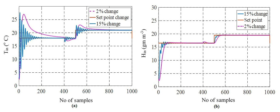
Figure 18(a) Graphical Representation of 2 % and 15 % Changes in Inlet Temperature Tin and (b) Graphical Representation of 2 % and 15 % Changes in Inlet Humidity Hin.
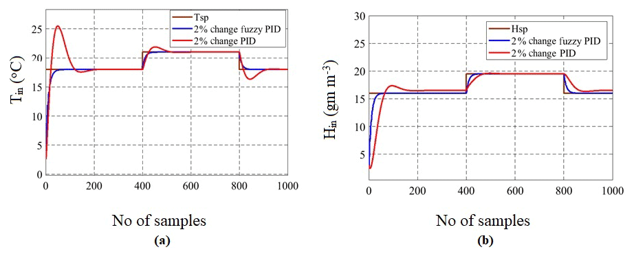
Figure 19(a) Comparison of 2 % Changes in Inlet Temperature Tin Using Fuzzy PID vs. PID Controllers and (b) Comparison of 2 % Changes in Inlet Humidity Hin Using Fuzzy PID vs. PID Controllers.
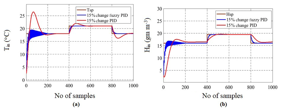
Figure 20(a) Comparison of 15 % Changes in Inlet Temperature Tin Using Fuzzy PID vs. PID Controllers and (b) Comparison of 15 % Changes in Inlet Humidity Hin Using Fuzzy PID vs. PID Controllers
Table 7 illustrates the comparative study of performance characteristics of the greenhouse model by applying variable step changes in the inlet temperature and inlet humidity with all the controllers. The primary objective of performing robustness analysis is to ensure that the controller works well in a real-time experimental setup of the greenhouse with different operating conditions. Although the settling time is of a satisfactory range, a large amount of peak overshoot and oscillatory response makes the controller weak, which could be avoided. Herein, the possible tuning of controller parameters can be limited to 2 % change to 15 % change for control of inlet temperature as well as inlet humidity while operating a commercial greenhouse.
Table 7Robustness analysis of PID controller for greenhouse system.
4.6 Stability Analysis of Greenhouse System with PI, PID and Fuzzy based PID Controllers
Stability in a system implies that any small changes in system input or system parameters do not result in large variations in system output. Therefore, stability is a crucial characteristic of the transient performance of a system (Nagrath and Gopal, 2006). The Bode plot is one of the most useful representations of the transfer function, which is a logarithmic plot comprising magnitude and phase angle plotted against frequency. Another method to analyze the stability of dynamical systems is Nyquist plot which is a frequency response method where open-loop equation G(jω)H(jω) is plotted with ω varying from zero to infinity. The graph obtained is Nyquist plot and if there are no encirclements around critical point () then the system is said to be stable (Susanto et al., 2018). The proposed work is focused on analyzing the stability of a greenhouse with the help of the Bode plot and Nyquist plot by applying 2 % and 15 % changes in the gain mentioned in Eqs. (4) to (7). The system should be able to accommodate these changes and reach a steady-state without deviating much from the original transfer function output response to reference tracking for 2 % changes in Tin.
In general, gain margin can be obtained by calculating vertical distance between the magnitude plot to x-axis at a frequency where the phase angle is 180∘. Similarly, phase margin is the vertical distance between the phase plot to x-axis at a frequency where the magnitude is 0 dB. The Bode plots illustrated in Figs. 21a, b, 22a and b shows that the system is stable with 2 % and 15 % changes in the inlet temperature Tin and inlet humidity Hin. The performance parameters of greenhouse in terms of gain margin and phase margin with 2 % and 15 % changes in temperature and humidity are shown in following Tables 8 and 9. Phase and gain margins are greater for 2 % changes in the operating condition, and they are stable. Also, from the above Bode plot, gain margin (GM) and phase margin (PM) for 2 % changes are positive at corresponding gain and phase crossover frequency of 0.0404 and 0.148 rad s−1, respectively. For 15 % changes, both GM and PM are also positive at frequencies 0.643 and 0.312 rad s−1, respectively. Therefore, as per the Bode stability criterion, the greenhouse is found to be stable for the given operating conditions. From the Bode plot, it is concluded that the greenhouse system is also stable with 15 % changes in the gain of four transfer functions given in Eqs. (4)–(7). From the above study, the climate CMS designed for commercial greenhouses has been tested using PID controllers. Various input scenarios have been tested for the desired humidity and temperature values. External disturbances have also been taken into consideration for the robustness analysis. Furthermore, climate control modules can provide a better result in irrigation control of commercial greenhouses in conjunction with CWSI. CMS arrangement has been tested in real-time scenario and should obtain the temperature and relative humidity fluctuations within the permissible limit for the plant growth. Temperature and humidity have been recorded in the short cycle of cucumber between 17 January 2019 to 4 February 2019. Fluctuation from the set point was within the acceptable limits. There is an average of temperature of 2.5 ∘C for a 9 m growth length and a relative humidity of 3.5 %. Information management systems to measure the data at any point of time have been previously investigated (Jahnavi and Ahamed, 2015); however, the same has been improved in the climate control strategy. CMS system can be further improved using permanent magnet direct current motors and the same has been previously verified using fuzzy logic systems (Sankardoss and Geethanjali, 2019).
Table 8Robustness analysis of inlet temperature for 2 % and 15 % changes in Tin.

Table 9Robustness analysis of inlet temperature for 2 % and 15 % changes in Hin.
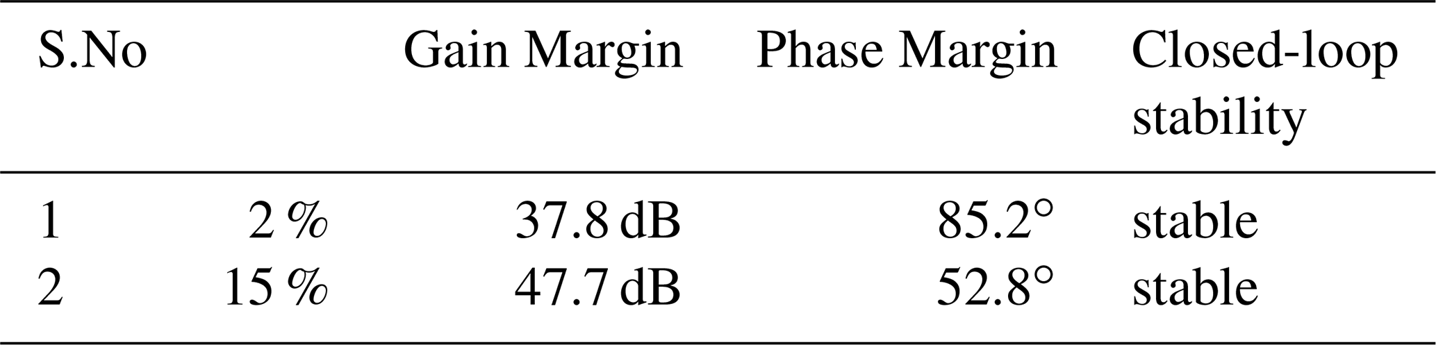
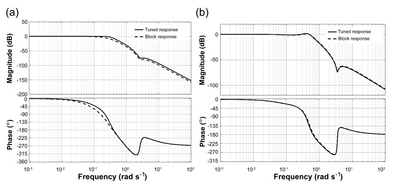
Figure 21(a) Stability Analysis using Bode Plot with Respect to Reference Tracking for 2 % Changes in Tin and (b) Stability Analysis using Bode Plot with Respect to Reference Tracking for 15 % Changes in Tin.
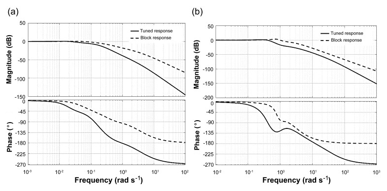
Figure 22(a) Stability Analysis using Bode Plot with Respect to Reference Tracking for 2 % Changes in Hin and (b) Stability Analysis using Bode Plot with Respect to Reference Tracking for 15 % Changes in Hin.
Further stability is analysed with the help of Nyquist plot for which pole-zero map has been plotted which is shown in Fig. 23. From the pole-zero map, it is inferred that system is stable because it has poles on the left-hand side of s plane (Martinez Baquero et al., 2018). The Nyquist stability criterion can be calculated from the formula mentioned in Eq. (15).
Where Z = number of roots of 1+G(s)H(s) in the right-hand side (RHS) of s-plane. N = number of encirclement of critical point 1+j0 in the clockwise direction. P = number of poles of open-loop transfer function (OLTF) in RHS of s-plane.
The Nyquist plot with 2 % and 15 % disturbances for greenhouse has been analysed to check the stability which is shown in Fig. 24a and b. From the figure, it can be seen that there are no encirclements around critical point so N=0 and also from the pole-zero map P=0. Therefore from Eq. (15), Z=0 which implies that even under disturbances greenhouse model is stable because there are no right side poles and also the system will be stable in the closed-loop (Salehi et al., 2019).
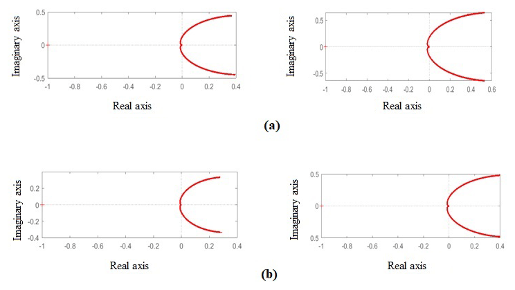
Figure 24(a) Stability Analysis using Nyquist Plot for Tin and Hin using PID Controller and (b) Stability Analysis using Nyquist Plot for Tin and Hin using Fuzzy Based PID Controller.
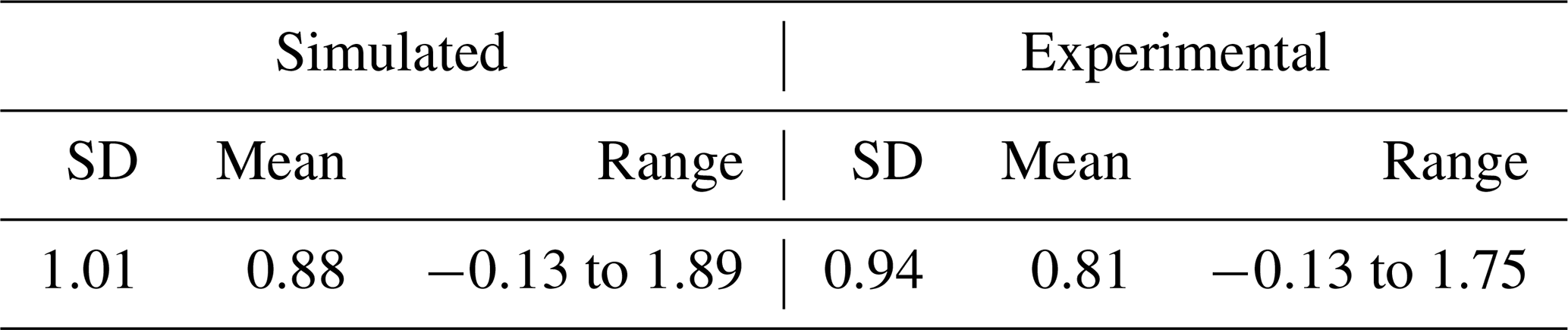
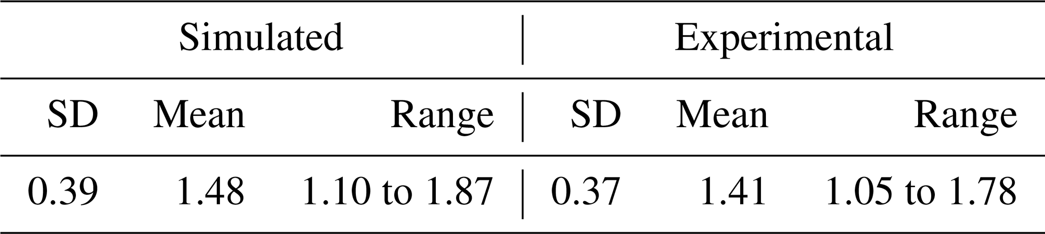
Table 11Temperature – Simulated verses experimental statistics.
4.7 Experimental Validation of Greenhouse Climate Control System
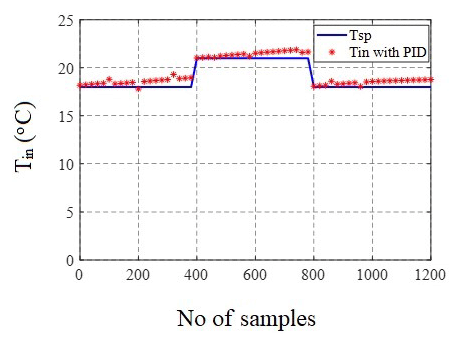
As discussed in Sect. 2 with respect to experimental setup PID controller was designed and implemented using Direct Digital Controller. The controller responses of humidity and temperature readings has been recorded for set points 16.5–19.5 g m−3 and 18–21 ∘C respectively. Figures 25 and 26 depicts the actual response obtained for two different time periods. It is observed that the controller performances are validated for both temperature and humidity variations. Standard deviations and mean for the humidity was 1.41 and 1.37 between the simulated and experimental with a mean of 17.48 and 17.43. Furthermore, the Standard deviations and mean for the temperature was 1.41 and 1.40 between the simulated and experimental with a mean of 18.98 and 19.48. The mean and standard deviation are found to be within the acceptable range as recorded in the Tables 10 and 11 for a particular sampling period.

Herein, the dynamic model has been developed for the greenhouse production process. Approximately 95 % of the process industries extensively use PID controllers remaining to their unpretentious architecture and for easy implementation. However, the regulation of several controllers in the commercial greenhouse environment is a challenge for process engineers and operators and still requires research attention because of varying disturbances and interaction variables. Herein, two PID loops for MIMO process were developed and effectively tuned to achieve stability and smooth output response. Robustness analysis was performed, and it was proven that with 2 %–5 % change in parameters, PID can achieve good with minimum peak overshoot, fast settling time, and less steady-state error and rise time. Stability analysis of greenhouse was performed to test the effectiveness of the designed CMS. Therefore, PID controllers are not limited to greenhouses but can be extended to other nonlinear applications. Climate CMS set up has been tested for one short cycle and the desired values have been verified within the permissible limit for the plant growth. It can be inferred from the simulation results that the non-interacting control scheme provides smooth set-point tracking and fast regulatory control even with disturbances. A comparative analysis between the experimental and simulated values has been carried out and the statistical data has been plotted in Figs. 25 and 26 and verified the standard deviation is within the range of 5 % to 10 %. Conventional timer-controlled systems controlled the water consumption in the earlier days and later on hydroponic irrigation system also controlled the water consumption as well as the most effective nutrient supply to the system. However automatic central control system based irrigation and fertigation systems clubbed with the climate control systems can provide more yield in the commercial greenhouse farming future innovations with this combinations to be studied in details to improve the climate control system strategy further. In the present study although smooth control action was achieved the tuning of the fuzzy rule-based system was complex and purely depends on expert knowledge. So this problem can be avoided with other soft computing tools like Genetic Algorithm (GA), Artificial Neural Networks (ANN) based predictive controllers which will be considered for future scope of work.
Data are available at https://doi.org/10.6084/m9.figshare.12738719 (Subin, 2020).
MCS has collected the experimental data required for the paper and contributed to the analytical modelling. AS has contributed to the MATLAB programming for the Modeling and Control system parts. VK has contributed to the conventional control system design and MATLAB programming part for the robustness analysis of the designed control system. RK has formulated the problem and designed Intelligent controller using the fuzzy-based control system. CP has overseen the activities.
The authors declare that they have no conflict of interest.
The authors are thankful to the establishments of Birla Institute of Technology and Science Pilani, Dubai campus for their support to conduct this research work and exclusively for the ABB Farm management, Al Khawaneej, Dubai for giving an opportunity by providing the live setups and facilities to carry out the experimental setup.
This paper was edited by Daniel Condurache and reviewed by three anonymous referees.
Adeyemi, O., Grove, I., Peets, S., Domun, Y., and Norton, T.: Dynamic neural network modelling of soil moisture content for predictive irrigation scheduling, Sensors, 18, 3408, https://doi.org/10.3390/s18103408, 2018.
Akkuzu, E., Kaya, U., Çamoğlu, G., Mengü, G. P., and Aşik, S.: Determination of crop water stress index and irrigation timing on olive trees using a handheld infrared thermometer, J. Irrig. Drain E.-ASCE, 139, 728–737, https://doi.org/10.1061/(ASCE)IR.1943-4774.0000623, 2013.
Alderfasi, A. A. and Nielsen, D. C.: Use of crop water stress index for monitoring water status and scheduling irrigation in wheat, Agr. Water Manage., 47, 69–75, https://doi.org/10.1016/S0378-3774(00)00096-2, 2001.
Alireza, A. and dos Santos Coelho, L.: A novel framework for optimization of a grid independent hybrid renewable energy system, A case study of Iran, Solar Energy, 112, 383–396, https://doi.org/10.1016/j.solener.2014.12.013, 2015.
Arruda, L. V. R., Swiech, M. C. S., Delgado, M. R. B., and Neves, F.: PID control of mimo process based on rank niching genetic algorithm, Appl. Intell., 29, 290–305, https://doi.org/10.1007/s10489-007-0095-6, 2008.
Bequette, B. W.: Process Control Modeling, Design and Simulation, Upper Saddle River, NJ Prentice Hall PTR, 2010.
Bilderback, T., Dole, J., and Sneed, R.: Water supply and water quality for nursery and greenhouse, North Carolina State University, Raleigh, NC, 1999.
Chang, W. D.: A multi-crossover genetic approach to multivariable PID controllers tuning, Expert Syst. Appl., 33, 620–626, https://doi.org/10.1016/j.eswa.2006.06.003, 2007.
Chaudhary, G., Kaur, S., Mehta, B., and Tewani, R.: Observer-based fuzzy and PID controlled smart greenhouse, Journal of Statistics and Management Systems, 22, 393–401, https://doi.org/10.1080/09720510.2019.1582880, 2019.
dos Santos Coelho, L. and Alireza, A.: An enhanced bat algorithm approach for reducing electrical power consumption of air conditioning systems based on differential operator, Appl. Therm. Eng., 99, 834–840, https://doi.org/10.1016/j.applthermaleng.2016.01.155, 2016.
Faccini Santoro, B., Rincón, D., Celleguin da Silva, V., and Mendoza, D. F.: Nonlinear model predictive control of a climatization system using rigorous nonlinear model, Comput. Chem. Eng., 125, 365–379, https://doi.org/10.1016/j.compchemeng.2019.03.014, 2019.
Faouzi, D., Bibi-Triki, B., Draoui, B., and Abene, A.: Modeling a Fuzzy Logic Controller to Simulate and Optimize the Greenhouse Microclimate Management using MATLAB SIMULINK, I. J. Mathematical Sciences and Computing, 3, 12–27, https://doi.org/10.5815/ijmsc.2017.03.02, 2017.
Hu, H. G., Xu, L. H., Zhu, B. K. and Wei, R. H.: A compatible control algorithm for greenhouse environment control based on MOCC strategy, Sensors, 11, 3281–3302, https://doi.org/10.3390/s110303281, 2011a.
Hu, H., Xu, L., Wei, R., and Zhu, B.: Multi-objective control optimization for greenhouse environment using evolutionary algorithms, Sensors, 11, 5792–5807, https://doi.org/10.3390/s110605792, 2011b.
Irmak, S., Haman, D. Z., and Bastug, R.: Determination of crop water stress index for irrigation timing and yield estimation of corn, Agron. J., 92, 1221–1227, https://doi.org/10.2134/agronj2000.9261221x, 2000.
Jahnavi, V. S. and Ahamed, S. F.: Smart wireless sensor network for the automated greenhouse, IETE J. Res., 61, 180–185, https://doi.org/10.1080/03772063.2014.999834, 2015.
Killingsworth, N. J. and Krstic, M.: PID tuning using extremum seeking, IEEE Contr. Syst. Mag., 26, 70–79, https://doi.org/10.1109/MCS.2006.1580155, 2006.
Kim, Y., Evans, R., Iversen, W., Pierce, R., and Chavez, J.: Software design for wireless in-field sensor-based irrigation management, in: Annual Meeting, American Society of Agricultural and Biological Engineers, paper No. 063074, Portland, OR, USA ,9–12 July, 2006.
Kittas, C., Karamanis, M., and Katsoulas, N.: Air temperature regime in a forced ventilated greenhouse with rose crop, Energ. Buildings, 37, 807–812, https://doi.org/10.1016/j.enbuild.2004.10.009, 2005.
Ljung, L.: System Identification: Theory for the User, 3rd Edn., PTR Prentice Hall, Englewood Cliffs, New Jersey, USA, 1987.
Martinez Baquero, J. E., Corredor Chavarr, F. A., and Jimenez Moreno, R.: Design of Controller PID and Stability Analysis for Drying of Corn's Grain, International Journal of Applied Engineering Research, 13, 15410–15416, 2018.
Marucci, A. and Cappuccini, A.: Dynamic photovoltaic greenhouse: Energy efficiency in clear sky conditions, Appl. Energ., 170, 362–376, https://doi.org/10.1016/j.apenergy.2016.02.138, 2016.
Meihui, L., Shangfeng, D., Lijun, C., and Yaofeng, H.: Greenhouse multi-variables control by using feedback linearization decoupling method, 2017 Chinese Automation Congress (CAC), Jinan, 604–608, 2017.
Nagrath, I. J. and Gopal, M.: Control Systems Engineering, New Age International Pvt Ltd, New Delhi, 2006.
Olenewa, J.: Guide to Wireless Communication, 3rd Edn., Cengage Learning, Boston, MA, 2013.
Pasgianos, G. D., Arvanitis, K. G., Polycarpou, P., and Sigrimis, N.: A nonlinear feedback technique for greenhouse environmental control, Comput. Electron. Agr., 40, 153–177, https://doi.org/10.1016/S0168-1699(03)00018-8, 2003.
Premkumar, K. and Manikandan, B. V.: Stability and Performance Analysis of ANFIS Tuned PID Based Speed Controller for Brushless DC Motor, Current Signal Transduction Therapy, 13, 19–30, 2018.
Pohlheim, H., Heibner Cunha, J. B., Couto, C., and Ruano, A. E. B.: A greenhouse climate multivariable predictive controller, ISHS Acta Hort., 534, 269–276, 2000.
Pucheta, J. A., Schugurensky, C., Fullana, R., Patino, H., and Kuchen, B.: Optimal greenhouse control of tomato-seedling crops, Comput. Electron. Agr., 50, 70–82, https://doi.org/10.1016/j.compag.2005.09.002, 2006.
Puglisi, G., Vox, G., Schettini, E., Morosinotto, G., and Campiotti, C.: Climate control inside a greenhouse by means of a solar cooling system, presented at the International Symposium on New Technologies for Environment Control, Energy-Saving and Crop Production in Greenhouse and Plant 1227, Beijing, China, 2017.
Saha, S., Monroe, A., and Dar, M. R.: Growth, yield, plant quality and nutrition of basil (Ocimum basilicum L.) under soilless agricultural systems, Ann. Agric. Sci., 61, 181–186, https://doi.org/10.1016/j.aoas.2016.10.001, 2016.
Salehi, A., Safarzadeh, O., and Hossein Kazemi, M.: Fractional order PID control of steam generator water level for nuclear steam supply systems, Nucl. Eng. Des., 342, 45–59, 2019.
Sankardoss, V. and Geethanjali, P.: Design and low-cost implementation of an electric wheelchair control, IETE J. Res., https://doi.org/10.1080/03772063.2019.1565951, 2019.
Subin, M.: Experimental data.zip, figshare, https://doi.org/10.6084/m9.figshare.12738719, 2020.
Susanto, A., Sampurno, and Suhardjono: Design of PLC Based Control System for Rotary Flexible Fixture with PID Compensator.IPTEK, J. Eng., 4, 26–32, 2018.
Teitel, M.: The effect of screened openings on greenhouse microclimate, Agr. Forest Meterol., 143, 159–175, https://doi.org/10.1016/j.agrformet.2007.01.005, 2007.
Trierweiler Ribeiro, G., Cocco Mariani, V., and dos Santos Coelho, L.: Enhanced ensemble structures using wavelet neural networks applied to short-term load forecasting, Intelligence, 82, 272–281, https://doi.org/10.1016/j.engappai.2019.03.012, 2019.
Zanetti Freire, R., dos Santos Coelho, L., dos Santos, G. H., and Cocco Mariani, V.: Predicting building's corners hygrothermal behavior by using a Fuzzy inference system combined with clustering and Kalman filter, Int. Commun. Heat Mass, 71, 225–233, https://doi.org/10.1016/j.icheatmasstransfer.2015.12.015, 2016.
Zhao, Z.-Y., Tomizuka, M., and Isaka, S.: Fuzzy gain scheduling of PID controllers, IEEE T. Syst. Man Cyb., 23, 1392–1398, 1993.