the Creative Commons Attribution 4.0 License.
the Creative Commons Attribution 4.0 License.
 | 09 Jul 2020
A teeth-discretized electromechanical model of a traveling-wave ultrasonic motor
Ning Chen
Dapeng Fan
This paper develops an electromechanical TWUSM (traveling-wave ultrasonic motor) model combining the driving circuit with the motor itself. An equivalent circuit model substituted for the piezoelectric ceramics is designed in the driving circuit model to obtain accurate input currents and powers. Then teeth discretization is implemented in the stator–rotor contact model, which can calculate the interaction forces more accurately. After building the complete model of TWUSM, a typical startup–stopping process is divided into five stages by evaluating the changes in contact status and driving forces. Finally, the fitness of transient responses of the rotor speed increasing from 55 % to 89 % shows that the proposed model fits better than the one without teeth discretization, and the experimental tests under various driving parameters verify the effectiveness of the model.
- Article
(4687 KB) - Full-text XML
- BibTeX
- EndNote


The TWUSM (traveling-wave ultrasonic motor) is the piezoelectric actuator which is excited near the resonant frequencies. The polarized piezoelectric ceramics of TWUSM are usually actuated by two alternating singular voltages. The stator particles change their displacements in space elliptical motion (Liu et al., 2019; Chen et al., 2018; Shi et al., 2018) with the deformations of piezoelectric elements. Several teeth are distributed along the circumferential direction to amplify the driving effect and deformed in accordance with the traveling wave (Renteria-Marquez et al., 2018). Therefore these motors present many significant merits compared to electromagnetic motors, for instance, rapid response, simple structure, and the capability of miniaturization (Zhang et al., 2016).
Because of the combination of piezoelectric actuation and friction drive, the TWUSM model attracts many researchers' attention. In general, their models can be divided into three types. First and most typical is the model stemming from Hagood and McFarland (1995), who assume the vibrating stator to be a two-freedom lumped spring-mass-damping system. However, the teeth discretization is ignored by only assuming the contact model to be continuous springs covering the ring area. The second type is proposed by Giraud et al. (2004), who imitate the d–q decomposition from the three-phase alternating current motor. Similarly, the ultrasonic motor is decomposed in the d–q coordinate, where d means the modal value and q represents the torque value. Jing (2015) develops Giraud's model by evaluating the modal vibration trajectory of the stator. However, the modal cannot be controlled accurately, like the external input such as the current or torque within the electromagnet motor. The third type is the semi-analytical model developed by Hagedorn et al. (1993) and Chen and Zhao (2005): they divide the stator into several parts according to the respective shape functions. Similarly, Bolborici et al. (2014) and Arturo (2016) model the stator and the rotor through the finite-volume-method model. Though the detailed model can analyze more microscopic details, it consumes vast computation sources and cannot achieve convergence all the time.
Besides these deficiencies, the above researchers simplify the model by idealizing the input signals as the ideal sinusoidal signals instead of deriving them from the driving circuit. The simplification not only deviates from reality, but also fails to detect the real-time currents. In this paper, a hybrid mechatronic model is proposed by combining the electrical system with the mechanical system. Besides, a more straightforward discretization strategy is adopted in the hybrid model to solve the problems of insufficient or excessive discretization, which can not only guarantee the accuracy, but also reduce the simulation nodes and calculation sources.
This paper is organized as follows. In Sect. 2, the principle of the ultrasonic motor is introduced. Then a hybrid model including the electrical circuit and the ultrasonic motor is built in the third section. In Sect. 4, the transient response and the contact status are studied under different torques to explore the microcosmic law. In Sect. 5, the integrated test system is built, and the simulation results under different parameters are verified from the comparisons of the experimental results.
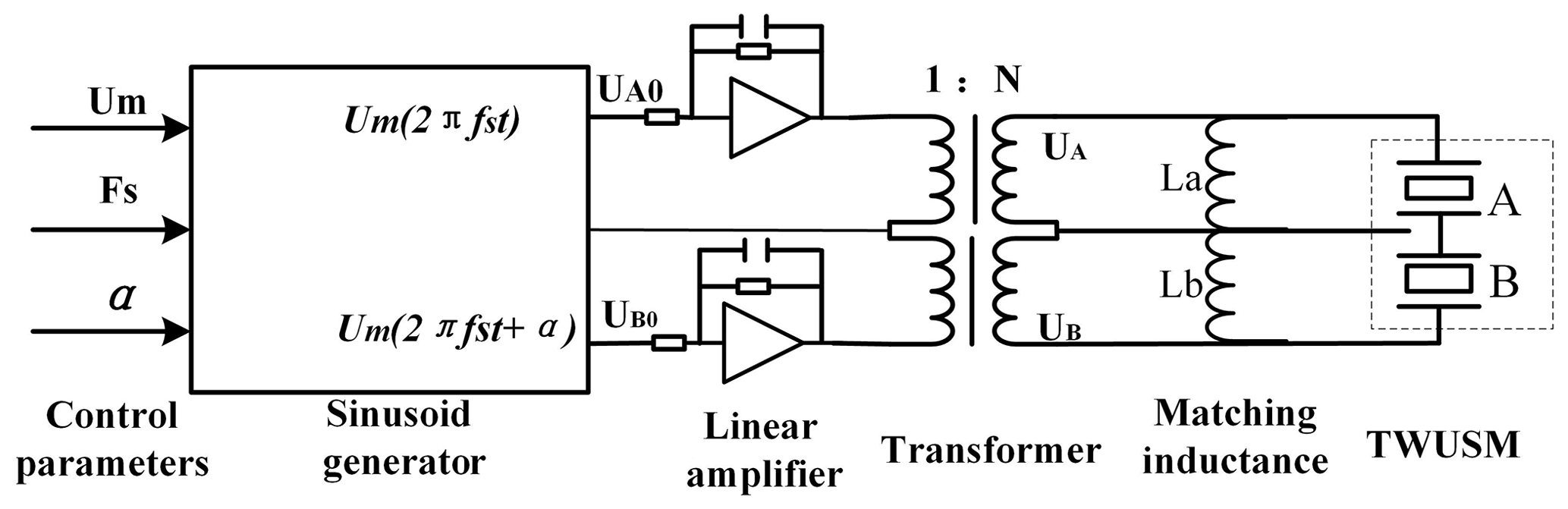
Figure 1 illustrates the working mechanism of the TWUSM. Piezoelectric ceramics are actuated by the two-phase sinusoidal voltages (UA and UB) determined by the amplitude (Um), frequency (f) and phase difference (α), as shown in Fig. 1a. It is evident that the two-channel input currents IA and IB can be informed by linking to the electrical network of the piezoelectric ceramics. Then the stator vibrates with the amplitude ξ during the transformation from the electrical energy to the mechanical energy, just like Fig. 1b. The modal responses of phase A and phase B are characterized as qA and qB, respectively. The stator's circumferential rotation propelled by the traveling wave drives the rotor via the friction interaction with the rotor. In Fig. 1c, Fpre represents the preload force, and Fz means the vertical force acting on the rotor. As shown in Fig. 1d, the output torque Tout is producing to overcome the applied torque Tload. Moreover, the whole rotor's mass and inertial are Mr and Jr, respectively.

Figure 1The block diagram of the TWUSM: (a) the driver; (b) the vibration and traveling wave of the stator; (c) the stator–rotor contact; (d) the rotor with the externally applied load.
The TWUSM prototype investigated in this paper is USR60-S3 (Shinsei Corp. Ltd, Japan), which works in the ninth vibration mode (N=9). So the natural vibration bending mode of the ring plate is denoted by B09. In USR60-S3, 90 teeth are distributed along the circumferential direction of the stator to improve overall driving capacities (Lin et al., 2002).
3.1 Modeling of the driving circuit
The driving circuit is supposed to generate pure sinusoidal waves for each fragment of the piezoelectric ceramics. Figure 2 illustrates the framework of the driving circuit actuated by three parameters (Um, Fs, α). The original sinusoid waves (UA0, UB0) are achieved by the two-channel waveform generators. Subsequently, the amplifying circuits and the transformers are assigned to produce the driving voltages. In terms of the capacitive characteristics of the piezoelectric segments, two inductors are placed in parallel to reduce the reactive power dissipation. Furthermore, in order to obtain the input voltages and currents, the circuit equivalent model (Fig. 3) is adopted to substitute for the piezoelectric ceramics (Mojallali et al., 2007).
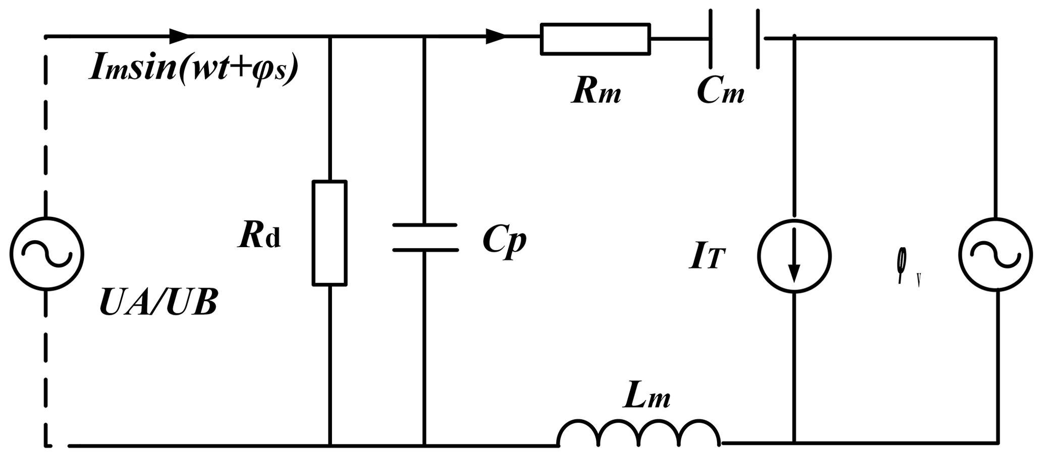
As shown in Fig. 3, Cp is the clamping capacitor of piezoelectric ceramics, whereby Rm, Cm and Lm represent equivalent resistance, equivalent capacitance and equivalent inductance, respectively. Rd means the resistance loss during the energy dissipation (Lu et al., 2011, 2020). The right element is the equivalent voltage ϕv, which describes the modal force derived from the stator–rotor contact model discussed in the next section. Finally, the current source IT represents the variation with the external load. It can be calculated from the proportion of the speed reduction caused by the applied torque. Its equation can be depicted as
Here, Ro is the middle radius of the stator; hs and hp are the thickness of the stator and the piezoelectric layer. kc is the mechatronic coupling coefficient which describes the speed drop versus the applied torque (Tload). When the maximum voltages and currents are Uam, Ubm, Iam and Ibm, the active input power of the two-phase piezoelectric ceramics can be calculated as
3.2 Modeling of the ultrasonic motor
3.2.1 Vibration model of the stator with a piezoelectric ring
In order to simplify the calculation, the vibration system (the piezoelectric elements and the stator) can be characterized as a 2-degree-of-freedom spring-mass-damping system. The modal coordinates (qA, qB) and the dynamic functions can be depicted as
where w=2πFs denotes the angular driving frequency, mo, do and ko represent modal mass, modal damping and modal stiffness, respectively, and ε is the imbalance coefficient between two-phase signals. Fd1 and Fd2 are the respective modal forces in both the tangential direction and the vertical direction. Besides, if λ is the wavelength of the traveling wave and , and are the eigenmode functions. When Φ(r) is the radial variance of this mode shape, the orthogonal modal shape function can be represented as
Thus, the vibration response of the stator stuck with the piezoceramics can be obtained by multiplying Eqs. (4) and (6); the result is depicted as
Finally, the tangential speed of the surface point can be derived. If h is the half-thickness of the stator and the middle radius of the stator is rp, whose radial variance is defined as ψav=Φ(rp), then the stator speed can be expressed as
3.2.2 Contact model with teeth discretization
Figure 4 illustrates the contact schematics of the motor with teeth discretization, and the stator–rotor contact model is built on the assumption that the rotor is rigid over all the contact areas, whereas the friction layer can be modeled as a series of linear springs. The yellow points mean the contact borders with the zone [], and the demarcation points between the traction zone and the braking zone are −x1 and x1.
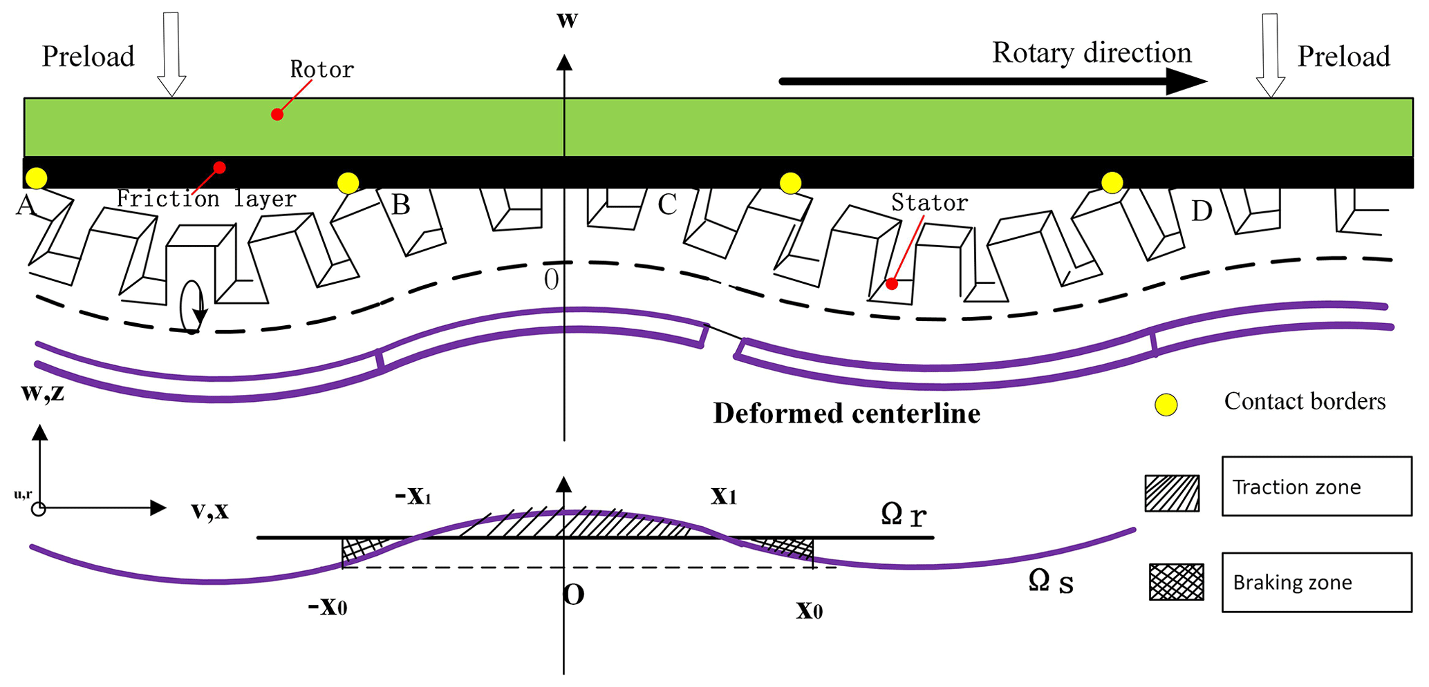
According to Fig. 4 and Eq. (9), the coordinates of contact border x0 and stick point x1 yield
where z(t) is the real-time vertical displacement of the rotor and means the rotor speed. When the joint stiffness of the dispersed springs is Kf, the unit pressure distributing from the contact interface to the stator can be given by
As shown in Fig. 5, every tooth can be simplified as a cuboid whose length and width are Rc and f, respectively. Since USR60 operates in ninth mode with 90 teeth, 10 teeth scatter in every wavelength. The coordinate plane OYZ is built on the central axis of the middle tooth, and the x axis is assigned along the traveling wave direction.
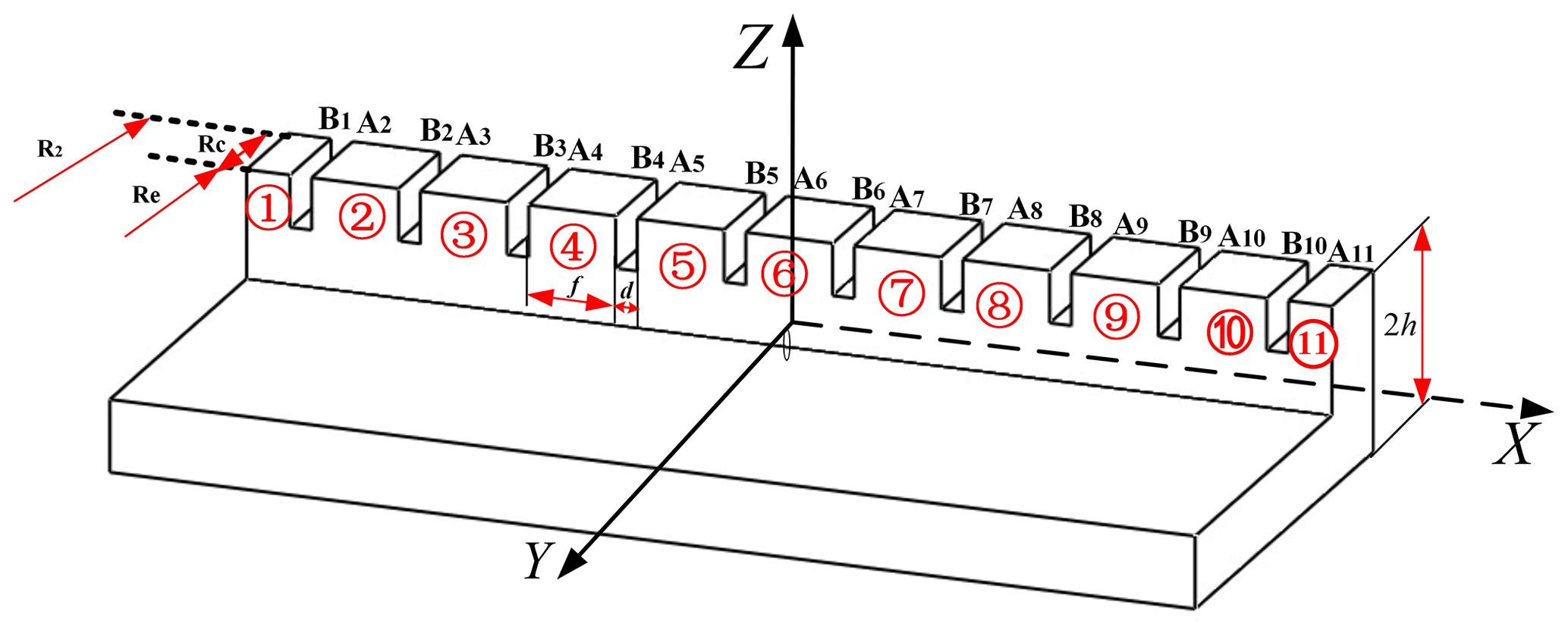
In succession, the left teeth edges are recorded as Aj, while the right ones are assigned as Bj. As shown in Fig. 5, the code numbers are named for every tooth, and only half of No. 1 and No. 11 are included in one wavelength. We define the gap width as d. Therefore every tooth position can be determined by its edge, whose horizontal coordinate and vertical coordinate are depicted as
Therefore, there are four cases when comparing the vertical coordinates with the stator half-thickness h. For convenience, the real contact boundaries are symbolized as s1, s2 with the following four cases.
- a.
If ZAj<h and ZBj<h, both edges of the tooth are apart from the contact area, and this tooth makes no contributions to the force generation.
- b.
If ZAj>h and ZBj>h, both the edges of the tooth are located in the contact area; therefore, , .
- c.
If ZAj>h and ZBj<h, the left edge of the tooth lies in the contact zone, and the intersection between the contact area and the tooth is just the right contact border; then, , s2j=x0.
- d.
If ZAj<h and ZBj>h, the right edge of the tooth is located in the contact region; similarly, , .
However, not all the particles of the contact region serve as the valid driving points. Whether the particles play the driving role needs the following detailed further discussions of stick–slip regional distribution, which also can be divided into four cases via the comparison between the contact borders and stick points.
- a.
If , both the stick points are in the contact area, the driving zone equals , and the blocking zones are and [x1, s2j].
- b.
If , the driving zone is [s1j, x1], while the blocking zone is [x1, s2j].
- c.
If , the driving zone is , while the blocking zone is .
- d.
If , all the particles share the driving effects.
Based on the above classifications, the interaction forces between the stator and the rotor become more accurate. First of all, the friction force FT can be derived from the integral operation of the whole teeth. Therefore FT(j) for every tooth can be expressed as Eqs. (15) and (16):
with
As shown in Eq. (18), the forces acting on the rotor along the axial direction can be calculated as Fz(j) without any classifications.
Moreover, the modal forces Fd1 and Fd2 consist of the vertical forcing vectors (Fdn1, Fdn2) and the tangential forcing vectors (Fdt1, Fdt2). The vertical parts can be calculated with the combination of modal matric and f(x). It can be expressed as Eqs. (19) and (20).
Similarly, the tangential forcing vectors from different areas can be read as Eqs. (21)–(25):
with
Finally, since the number of traveling waves is 9, the force results of the whole motor can be derived by summarizing the above calculated results. In the end, the whole force vector can be depicted as
3.2.3 The whole motor model
In terms of the whole TWUSM, the vertical displacement and the rotational velocity of the rotor can be described in the third and fourth functions in Eq. (27), where dz represents the vertical damping and dr means the rotational damping. Finally, the final analytical model can be depicted as
It should be emphasized that the bridges between the circuit model and the motor model are the equivalent electrical voltages (φva,φvb), which can be expressed as Eq. (28). The efficiency ηe from the input power to the output power can be depicted as Eq. (29), which is used to evaluate the energy utilization factors with variable loads.
The total model covering the elements in Fig. 1 is built in the Simulink platform, with the parameters listed in Appendix A. In order to obtain more microscopic properties, simulations are implemented on the transient response without load and the contact status under different torques.
4.1 Transient response without load
Figure 6 displays the startup–stopping response of the TWUSM when the input signals are the sinusoid waves containing 800 periods and the amplitude Um and the frequency Fs are 1 V and 43 kHz, respectively. The simulating signals cover the main electromechanical parameters discussed in Eqs. (10), (11) and (27).
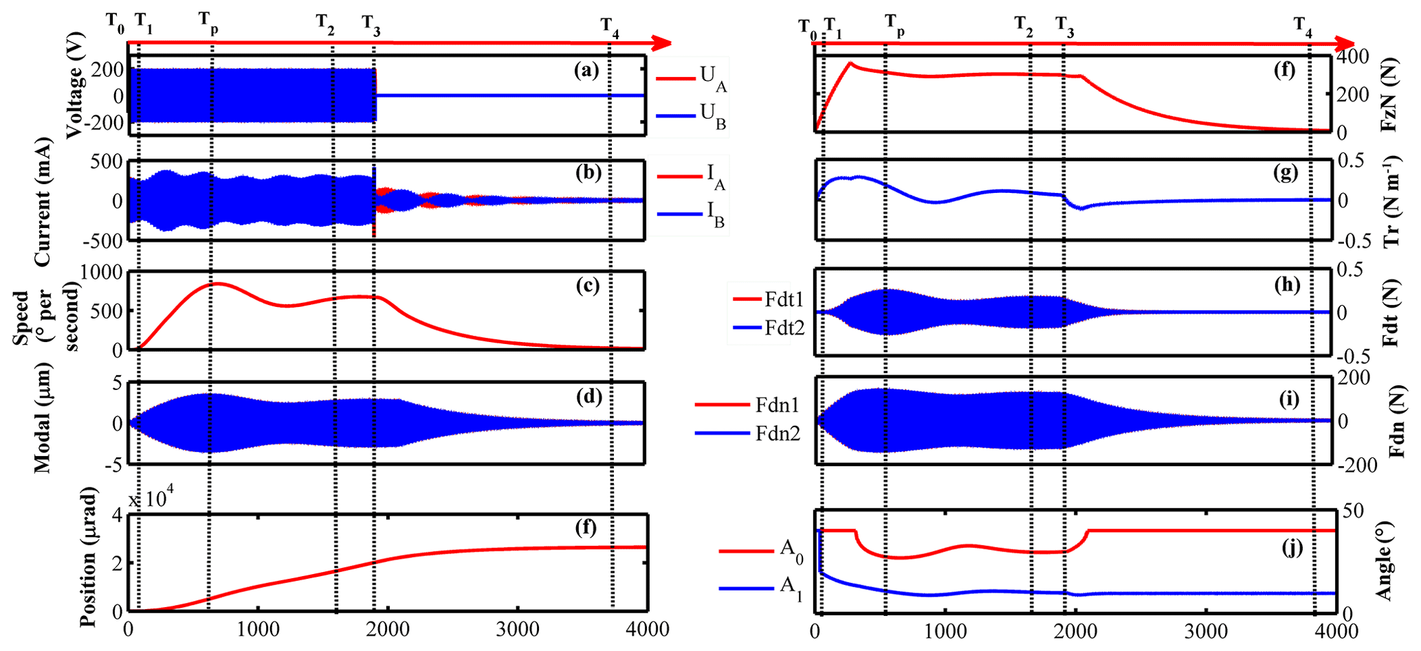
Figure 6Transient response of the unloaded motor with the driving signals containing 800 periods of activation: (a) the two-phase input voltages, (b) the vertical force applied in the rotor, (c) two-phase input currents, (d) the output torque, (e) the two-phase vibration response, (f) the tangential modal forces, (g) the revolving speed, (h) the vertical modal forces, (i) the rotor angle, and (j) the contact parameters.
There are five stages, including the pre-static stage [T0, T1], dynamic-friction and fluctuation stage [T1, T2], stabilized stage [T2, T3], vibration decay stage [T3, T4] and self-locking stage [T4, T5]. At the pre-static stage, the force generation between the stator and the rotor cannot overcome the static friction; therefore, the rotor stays motionless. Once the motor comes into the dynamic-friction stage, the vibration amplitude ξ (Fig. 6d) increases, accompanied by the ascending modal forces. The contact status changes from full contact to partial contact. However, the effective driving zone (Fig. 6j) shrinks, and the number of teeth involved in contact or driving also changes periodically, which causes the continuous fluctuation of the input currents (Fig. 6b). When the motor steps into the steady stage, the vibration amplitude and the driving zone become steady. Until the moment that the driving signals are withdrawn, the contact zone extends again and returns to the full-contact status before locking the rotor. At this time, the sustaining driving zone supports the final decaying process. The results also indicate that the proposed comprehensive integration model expands our understanding of the internal microcosmic law of the TWUSM, which is useful for the motor's stepwise position control.
4.2 Contact status with load
Figure 7 proposes the contact status of the teeth in a 40∘ circumferential range when the torque is 0.5 N m. It can be observed that the stick points are all located inside the contact zones, and only No. 5, No. 6 and No. 7 of the teeth are in full-contact status. The other teeth are out of contact and make no contribution to force generation. Besides, Fig. 7b shows the contact parameters when the torque is increased. The driving zone becomes wider, while the length of the contact zone remains constant, which means more teeth are added to the driving range to overcome the increased torque.
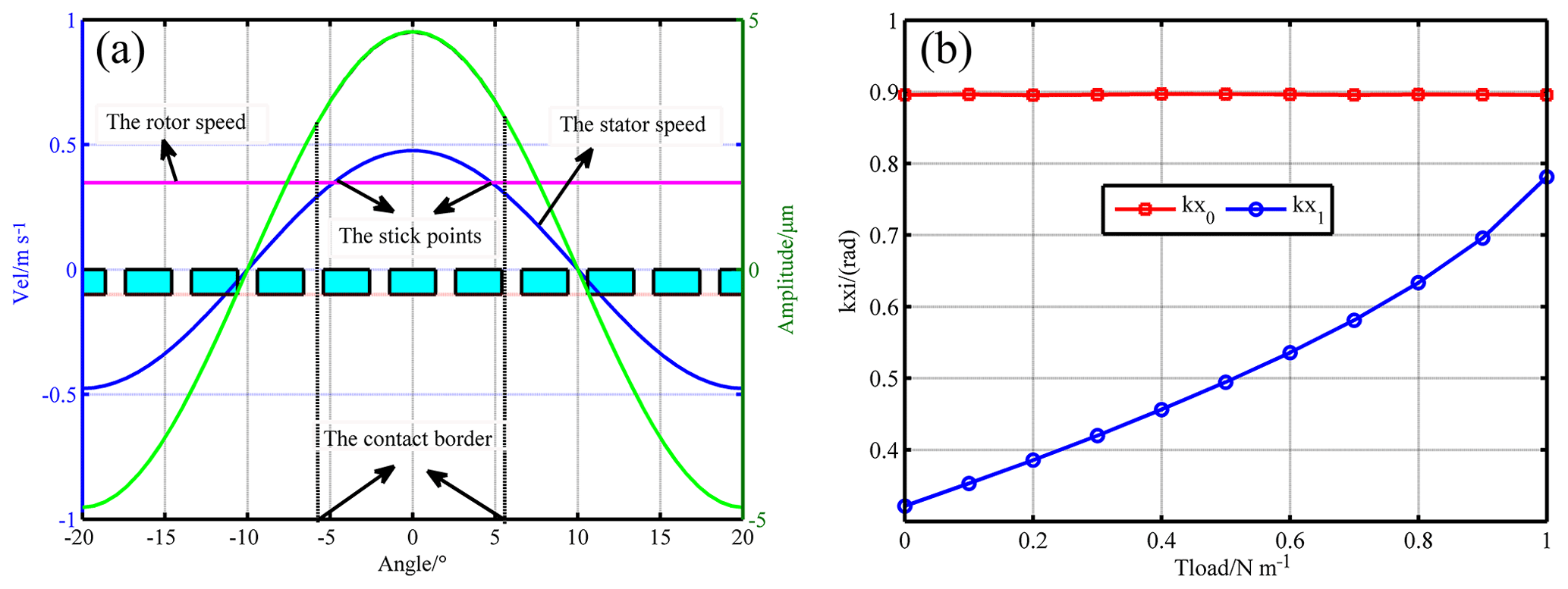
Figure 7The contact status: (a) the external torque is 0.5 N m; (b) the contact parameters under different torques.
5.1 Experimental setup
Figure 8 displays the integrated measurement system that consists of the driving circuit, the mechanical platform, the FPGA board (National Instruments Corp, USA), and the dSPACE1103 control board (dSPACE Corp, Germany). There is an incremental encoder AFS60A (SICK Corp, Germany) which has 65 536 lines. The external load is generated by a torque motor with the maximum torque 1 N m. The dSPACE1103 also generates the input parameters (Um, Fs, α) which output to the FPGA (field programmable gate array) board to generate the sinusoidal signals (UA0 UB0). When the motor is actuated, the currents (IA1,IB1) of the piezoelectric ceramics are measured by hall sensors (Zhonghuo Sensing Corp, PRC) and the voltages (UA1, UB1) are measured by voltage transformers (Zhonghuo Sensing Corp, PRC). Then, the signals are all processing in the FPGA board and transformed into the amplitude (Iam, Ibm, Uam, Ubm) and the phase differences (φa, φb). Therefore the input powers (PA, PB) can be obtained from Eqs. (2) and (3). Finally, we can get the motor efficiency according to Eq. (29). The experimental platform integrates the function of flexible adjustment and online calculation. Therefore parameter identification and performance evaluation can be realized in high efficiency.

5.2 Experiment results
5.2.1 The startup response
As shown in Fig. 9, when the amplitude Um is 1.3 V and the frequency Fs is 41.5 kHz, the startup velocity curves with or without teeth discretization are compared. As can be seen, the results with the teeth discretization method achieve better fitness. The fitness is 55 % if the teeth structure is ignored, and the fitness increases to 89 % when the teeth discretization is implemented. Moreover, the 2 ms delay which occurs in the results without the teeth discretization model disappears with the proposed model. This can be explained by eliminating the driving effect of the tooth gap by refining the interaction forces and the contact status. Furthermore, the contact area which has been limited to the teeth space rather than the whole ring is closer to reality. Furthermore, the startup speed responses actuated by various frequencies, and a certain amplitude, are displayed in Fig. 10a. To gain more detailed observations, the speed curves before 5 ms are displayed in Fig. 10b. All results under different frequencies show good agreements between the numerical results and experimental ones and the differences of the response process. Figure 10b indicates that the motor starts more quickly and obtains less overshoot with the increasing frequency.
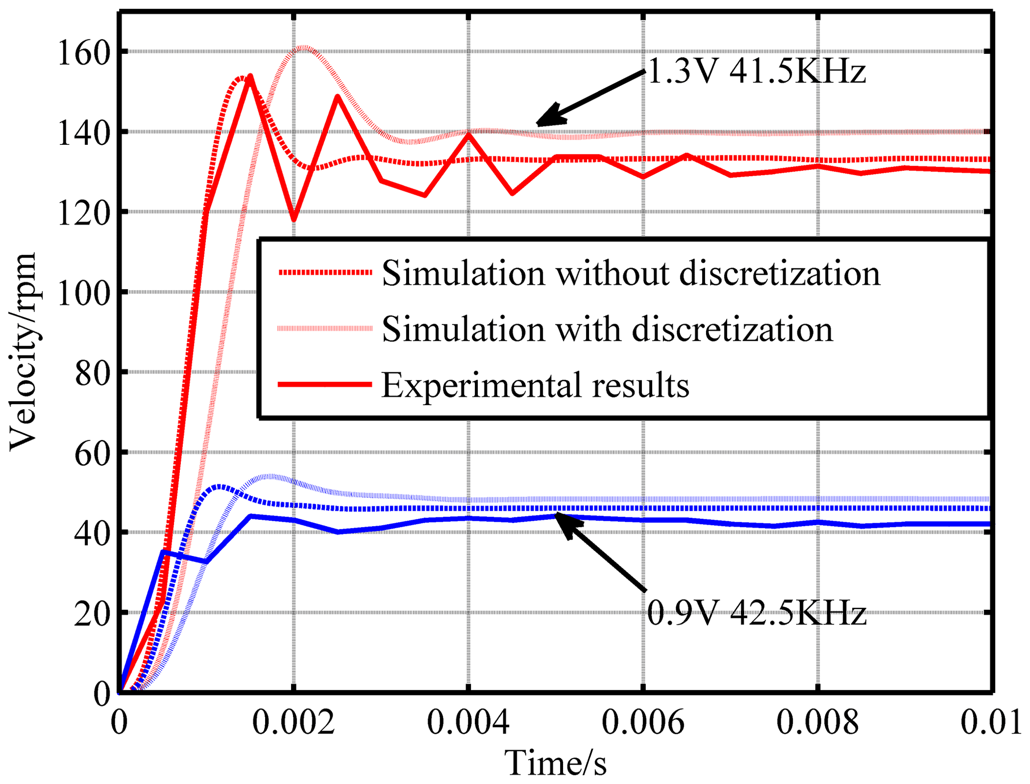
Figure 9The transient characteristics comparing the experiment results and simulation results with or without the teeth discretization.

Figure 10Comparison between simulation results and experimental ones when the amplitude is 1 V: (a) the step response within 20 ms; (b) the step response within 5 ms.
5.2.2 Speed performances under different driving parameters
Due to the complexity of piezoelectric ceramics, the vibration conditions are different in diverse regions before or after the resonant points. In order to obtain the ideal working range, especially the frequency interval of the proposed integrated model, the rotor velocities of different amplitudes and frequencies are displayed in Fig. 11a and b.
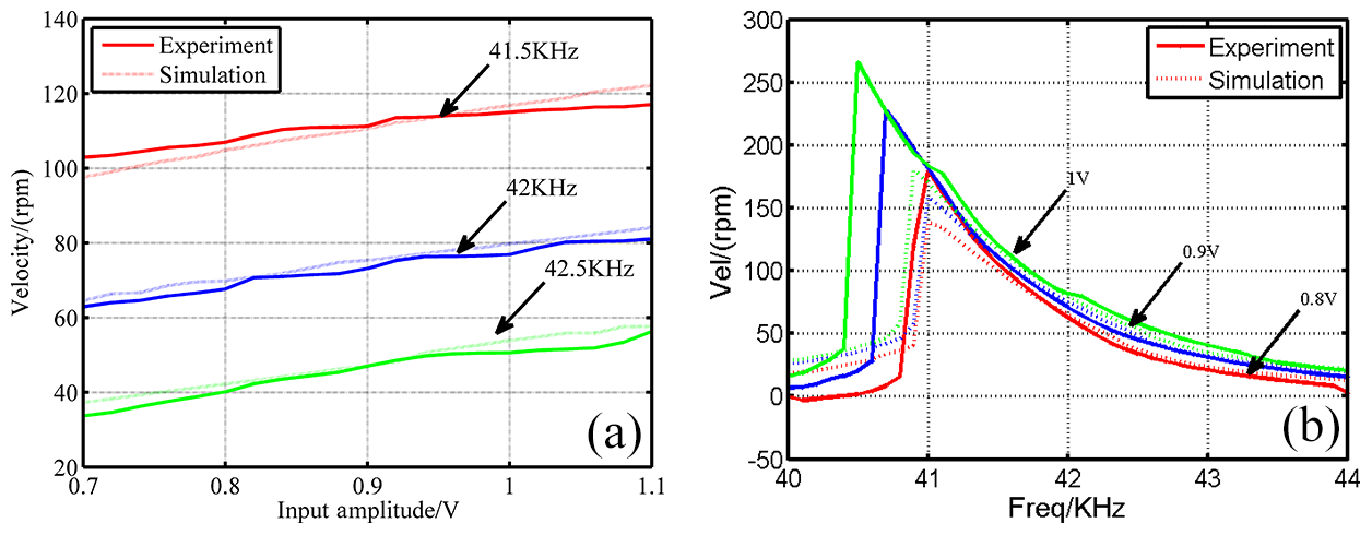
Figure 11Velocity response under different driving parameters: (a) speed versus amplitude; (b) speed versus frequency.
It can be seen from Fig. 11a that the linearity between the driving amplitudes and the rotor speed is evident on the whole. And Fig. 11b demonstrates that the speed gradually increases and then drops to a lower value when the frequency is changed from 40 to 44 kHz. Moreover, the frequencies located on the peak velocity decrease as the amplitude increases. This is due to the variation of the natural frequency of the stator caused by the softening nonlinearity. We can conclude that when the frequency comes close to the resonant frequency, the simulation model cannot describe the speed adequately, which may result from the simplification of the stator modal model, as the frequency higher than the resonant peak is usually chosen as the working range, where the fitness becomes better especially from 41 and 44 kHz. The effective fitting results further prove the feasibility of the proposed model.
In all, the above test of speed performances with two driving parameters verifies the validity of the model located in a specific working area, where the amplitude is higher than 0.7 V and the frequency is higher than 41 kHz.
5.2.3 The mechanical characteristics
In order to verify the model in the functions of external load, Fig. 12 illustrates the comparison of mechanical characteristics from the simulations and the experiments. As can be seen, the velocity–torque curve exists in good agreement within the frequencies from 42 to 43 kHz, while the results occur with a little error with the lower frequency. Also, we can observe that the efficiency becomes higher when the frequency is near the resonant value, and the optimal torque we should impose on the motor will be less than 0.5 N m.

Figure 12Comparison of the mechanical characteristics between simulation and experimentation: (a) 0.9 V, 41.5 kHz; (b) 1 V, 41.5 kHz; (c) 1.3 V, 42 kHz; (d) 1.3 V, 42.5 kHz.
This paper presents an electromechanical hybrid model that combines the driving circuit and the TWUSM itself. The main work and contributions can be listed as follows.
-
A driving circuit model combining the circuit components with the load-dependent equivalent circuit model is proposed to simulate the real electric network, which not only supports the TWUSM model, but also helps to gain the input voltages and currents for the calculation of input power.
-
The teeth discretized method is employed to refine the contact status and interaction forces limited to the teeth space, which improves the accuracy of the rotor step response not only in the rising time, but also the steady value.
-
Model agreements are tested on the rotor speed under different parameters (amplitude, frequency, and torque) based on a multi-parameter test system, which demonstrates the feasibility and effectiveness within the ideal frequency working range higher than the resonant frequency.
Moreover, the proposed model achieves the observation of the microscopic characteristics like input currents and vibration response of the transient startup–stopping operation, which are of great significance for precise control of micro-stepping of the TWUSM in the future.
The data generated during this study are available from the corresponding author on reasonable request.
NC contributed to this work with the building of the integrated measurement system and the analysis from simulation and experiment; DF contributed to the guidance of the research and the revision of the manuscript.
The authors declare that they have no conflict of interest.
The authors are grateful for the financial support from the National Basic Research Program of China (973 Program, grant no. 2015CB057503).
This research has been supported by the National Basic Research Program of China (973 Program (grant no. 2015CB057503)).
This paper was edited by Daniel Condurache and reviewed by two anonymous referees.
Arturo, I.: Modeling of piezoelectric traveling wave rotary ultrasonic motors with the finite volume method, The University of Texas, El Paso, 2016.
Bolborici, V., Dawson, F. P., and Pugh, M. C.: A finite volume method and experimental study of a stator of a piezoelectric traveling wave rotary ultrasonic motor, Ultrasonics, 54, 809–820, 2014.
Chen, C. and Zhao, C.: Modeling of the stator of the traveling wave rotary ultrasonic motor based on substructural modal synthesis method, Journal of Vibration Engineering, 18, 238–245, 2005.
Chen, N., Chao, Q., Zheng, J. J., Fan, D. P., and Fan, S. X.: Impedance Characteristics Test of Ultrasonic motor Based on Labview and FPGA, CSAA/IET International Conference on Aircraft Utility Systems, Guiyang, China, https://doi.org/10.1049/cp.2018.0352, 2018.
Giraud, F., Semail, B., and Audren, J. T.: Analysis and phase control of a piezoelectric traveling-wave ultrasonic motor for haptic stick application, IEEE T. Ind. Appl., 40, 1541–1549, 2004.
Hagedorn, P., Wallaschek, J., and Konrad, W.: Travelling wave ultrasonic motors, part II a numerical method for the flexural vibrations of the stator, J. Sound Vib., 168, 115–122, 1993.
Hagood IV, N. W. and McFarland, A. J.: Modeling of a Piezoelectric Rotary Ultrasonic Motor, IEEE T. Ultrason. Ferr., 42, 210–224, 1995.
Jing, K.: TWUSM dynamic modeling and the optimal control of vibration mode vector, Hebei University of Technology, Hebei Province, China, 2015.
Lin, F. J., Duan, R. Y., Wai, R. J., and Hong, C. M.: LLCC resonant inverter for piezoelectric ultrasonic motor drive, IEEE Proceedings – Electric Power Applications, 146, 479–487, 2002.
Liu, J., Niu, Z. J., Zhu, H., and Zhao, C. C.: Design and Experiment of a Large-Aperture Hollow Traveling Wave Ultrasonic Motor with Low Speed and High Torque, Appl. Sci., 9, 1–16, 2019.
Lu, X., Hu, J., and Zhao, C.: Analyses of the temperature field of traveling-wave rotary ultrasonic motors, IEEE T. Ultrason. Ferr., 58, 2708–2719, 2011.
Lu, X., Wang, Z., Shen, H., Zhao, K., Pan, T., and Kong, D.: A Novel Dual-Rotor Ultrasonic Motor for Underwater Propulsion, Appl. Sci., 10, 31, https://doi.org/10.3390/app10010031, 2020.
Mojallali, H., Amini, R., Izadi-Zamanabadi, R., and Jalali, A. A.: Systematic experimental based modeling of a rotary piezoelectric ultrasonic motor, ISA T., 46, 31–40, 2007.
Renteria-Marquez, I. A., Renteria-Marquez, A., and Tseng, B. T. L.: A novel contact model of piezoelectric traveling wave rotary ultrasonic motors with the finite volume method, Ultrasonics, 90, 5–17, 2018.
Shi, W. J., Zhao, H., Ma, J., and Yao, Y.: Dead-zone compensation of an ultrasonic motor using an adaptive dither, IEEE Transactions on Industrial Electronics, 65, 3730–3739, 2018.
Zhang, Y., Qu, J., and Wang, H.: Wear Characteristics of Metallic Counterparts under Elliptical-Locus Ultrasonic Vibration, Appl. Sci., 6, 289, https://doi.org/10.3390/app6100289, 2016.