A Bayesian-optimized convolutional neural network bidirectional gated recurrent unit model for dynamometer card reconstruction in beam pumping units

The surface dynamometer card (DC) of beam pumping units plays a critical role in monitoring well conditions and adjusting pumping parameters. While several data-driven approaches based on deep learning have been applied to this task, they often suffer from limitations in input data completeness, model tuning, and the effective integration of deep learning structures. To address these issues, this paper proposes a novel inversion model named BO-CNN-BiGRU, which combines convolutional neural networks (CNNs), bidirectional gated recurrent units (BiGRUs), and Bayesian optimization (BO). The model inputs are determined based on the mechanism of beam pumping systems. CNNs are used to extract deep spatial features from electrical signals, BiGRU captures complex temporal dependencies to reconstruct polished-rod load curves, and BO enables automatic hyperparameter optimization. Field experiments conducted using real oil well production data demonstrate that the BO-CNN-BiGRU model achieves superior accuracy, robustness, and practicality. The proposed method can provide more reliable indicator diagrams to support intelligent regulation and diagnosis of beam pumping operations.

1 Introduction

The dynamometer card is a closed-loop graph constructed from the relationship between the polished-rod load and the polished-rod displacement. It reflects the operating conditions of downhole equipment such as the sucker rod column and pump. In actual oilfield production, the dynamometer card serves as a primary basis for analyzing downhole conditions and well productivity and for adjusting pumping unit parameters. Currently, the majority of oil wells use remote terminal unit (RTU) systems to measure dynamometer cards. However, the load sensors commonly used in these systems have low reliability and are prone to drift. These sensors require frequent calibration and replacement to maintain accuracy (Wang et al., 2018; Lindh et al., 2015), leading to waste of human and material resources. Therefore, real-time measurement of the dynamometer card without load sensors holds significant engineering value (Yang et al., 2014).

Three-phase asynchronous motors are commonly used as the power source for pumping units in oil fields. Electrical parameters serve as important reference variables that directly reflect the operating conditions of the pumping units. Compared to load sensors, electrical parameter sensors are more reliable, accurate, and easier to install. Over the years, the academic community has focused on researching methods for indirectly obtaining dynamometer cards through motor electrical parameters. A common approach is to establish a physical calculation model of the pumping unit system (Gibbs, 1987; Yin et al., 2022); however, this approach involves complex integrated characteristics such as mechanical vibration, dynamic load, friction, and the elastic sliding of belt transmission, resulting in significant calculation errors (Zheng et al., 2019). Additionally, these physical models require a large number of parameters to be measured, leading to substantial economic and technical limitations in practical applications. In recent years, data-driven methods based on deep learning (DL) have been widely used. Unlike physical modeling, this method only requires the preparation of the necessary dataset after determining the appropriate DL model, eliminating the need for the physical modeling process. These characteristics make DL particularly effective when handling complex tasks or physical models that are difficult to compute (Lee et al., 2023). With the construction of digital oil fields, there is a vast amount of untapped valuable data on site, providing a data foundation for data-driven methods. Current methods include hybrid modeling methods based on physical models and data-dependent kernel online sequential extreme learning machines (Wei and Gao, 2018), as well as algorithms that incorporate physical significance (Wang et al., 2019), such as backpropagation (BP) neural networks and convolutional neural networks (CNNs) (Di Mauro et al., 2024).

Although existing research has made significant contributions to the inversion of dynamometer cards, certain limitations remain. Many of these data-driven models adopt a single deep learning (DL) architecture to establish a mapping between motor output power and polished-rod load, while the polished-rod displacement still needs to be indirectly obtained by measuring the crank angle of the pumping unit. Furthermore, dynamometer card inversion is essentially a time series prediction problem as it involves estimating future values from sequentially ordered observations; however, this temporal nature has not been adequately considered in previous studies. Given the multiple influencing factors affecting polished-rod load, modeling based on a single information source often suffers from incomplete input data, which limits prediction accuracy and increases output error (Chen and Guan, 2023). To overcome the limitations of single-model performance, hybrid models that integrate multiple deep learning modules have gained widespread application (Bayoudh, 2024). These models leverage the inherent strengths of different neural network architectures to effectively enhance overall model performance. Among DL models, convolutional neural networks (CNNs) have demonstrated strong capabilities in extracting deep features. However, CNNs are primarily designed for static data processing and lack the ability to capture long-term temporal dependencies in sequential data. This structural limitation restricts their effectiveness when dealing with long time series sequences (Xing et al., 2020). In contrast, bidirectional gated recurrent units (BiGRUs), which incorporate memory units, gating mechanisms, and bidirectional processing, can effectively learn the temporal correlations between input sequences (Teng et al., 2021).

Although data-driven methods based on deep learning (DL) are well-suited for solving such problems, achieving satisfactory prediction performance requires a specialized understanding and careful tuning of network depth and related parameters. First, different combinations of hyperparameters significantly impact model performance, yet the relationship between hyperparameters and performance often behaves like a black box (Avendaño-Valencia et al., 2021). Second, it is unrealistic to expect a model trained on a specific dataset to perform optimally across all unique datasets (Zhang et al., 2022). Traditional methods such as grid search and random search manually set hyperparameter values during training, requiring substantial time and multiple iterations to identify optimal parameters. Moreover, the interdependence among parameters makes it difficult to determine the best adjustment direction (Fang et al., 2024). In contrast, Bayesian optimization (BO) is capable of solving complex optimization problems with unknown objective function expressions. It can find the optimal solution of the target function with minimal computation and a relatively small number of samples, making it particularly well-suited for automatic hyperparameter tuning in deep learning (Lee et al., 2021; Chen et al., 2023).

Based on this, a hybrid model that integrates Bayesian optimization (BO), convolutional neural networks (CNNs), and bidirectional gated recurrent units (BiGRUs) is selected for the analysis of dynamometer cards from beam pumping units. Owing to its excellent performance, the model has seen widespread application. CNNs are utilized for their superior capability in feature extraction to perform fused extraction of input data features. The extracted deep features are then processed in a temporal sequence by BiGRUs to construct a model for inferring the polished-rod load. Bayesian optimization is employed to optimize hyperparameters, thereby enhancing the model's efficiency and accuracy. Experimental results based on real-world data from the Xinjiang oilfield demonstrate that the proposed model exhibits robust dynamometer card inversion capability.

2 Selection of model input variables

The data-driven modeling approach employed by deep learning methods places high demands on the validity and representativeness of input data. Appropriate selection of input variables is therefore essential for improving both model accuracy and generalization capability. In this study, dynamic input parameters are determined from a dual perspective that combines the pumping unit mechanism model with the completeness of the available input data. This strategy aims to enhance the adaptability and predictive reliability of the proposed model, ensuring closer consistency with the actual operating behavior of the pumping system.

As demonstrated by the mechanism-based indicator diagram inversion model using electrical parameters, the suspension point load model involves variables such as the beam angle and electrical power. Once the structural and dynamic parameters of the pumping unit system are determined and the model is trained, these parameters are implicitly embedded and fixed in the weights and biases of the deep learning model. Therefore, the key input variables are the beam crank angle (θ) and the actual electrical power (p_act). These two variables must be included as input features in the proposed model. In addition, based on the electromagnetic torque (T_e) of the motor and the rotor motion equation,

$$\begin{array}{}\text{(1)}& \left\{\begin{array}{l}{T}_{\mathrm{e}}=\frac{p_{\mathrm{0}}}{\mathrm{2}}\mathit{i}\frac{\partial \mathbf{L}}{\partial \mathrm{\Omega }}{\mathit{i}}^T\\ J_{\mathrm{1}}\frac{\mathrm{d}{\mathit{\omega }}_{\mathrm{1}}}{\mathrm{d}t}=T_{\mathrm{e}}-T_{\mathrm{L}}-\mathit{\mu }{\mathit{\omega }}_{\mathrm{1}}\end{array}.\right.\end{array}$$

In the above equation, P₀ denotes the number of pole pairs of the motor, i represents the current vector, L is the inductance and mutual inductance matrix, Ω denotes the rotor position angle, J₁ is the moment of inertia of the rotor, ω₁ is the angular velocity, T_L is the load torque, and μ represents the friction coefficient.

Based on Eq. (1), the load torque T_L can be expressed as follows:

$$\begin{array}{}\text{(2)}& T_{\mathrm{L}}={\displaystyle \frac{p_{\mathrm{0}}}{\mathrm{2}}}\mathit{i}{\displaystyle \frac{\partial \mathbf{L}}{\partial \mathrm{\Omega }}}{\mathit{i}}^T-J_{\mathrm{1}}{{\displaystyle \frac{\mathrm{d}{\mathit{\omega }}_{\mathrm{1}}}{\mathrm{d}t}}}_{\mathrm{L}}-\mathit{\mu }{\mathit{\omega }}_{\mathrm{1}}.\end{array}$$

As indicated by the above equation, the current also reflects the magnitude of the motor load torque. Therefore, to further improve the completeness of the input data, the motor current (I) is additionally introduced as an input variable, alongside the beam crank angle (θ) and actual electrical power (p_act). Since motor current is also an electrical parameter, its inclusion requires only one additional measurement, which does not significantly increase the complexity or difficulty of data acquisition.

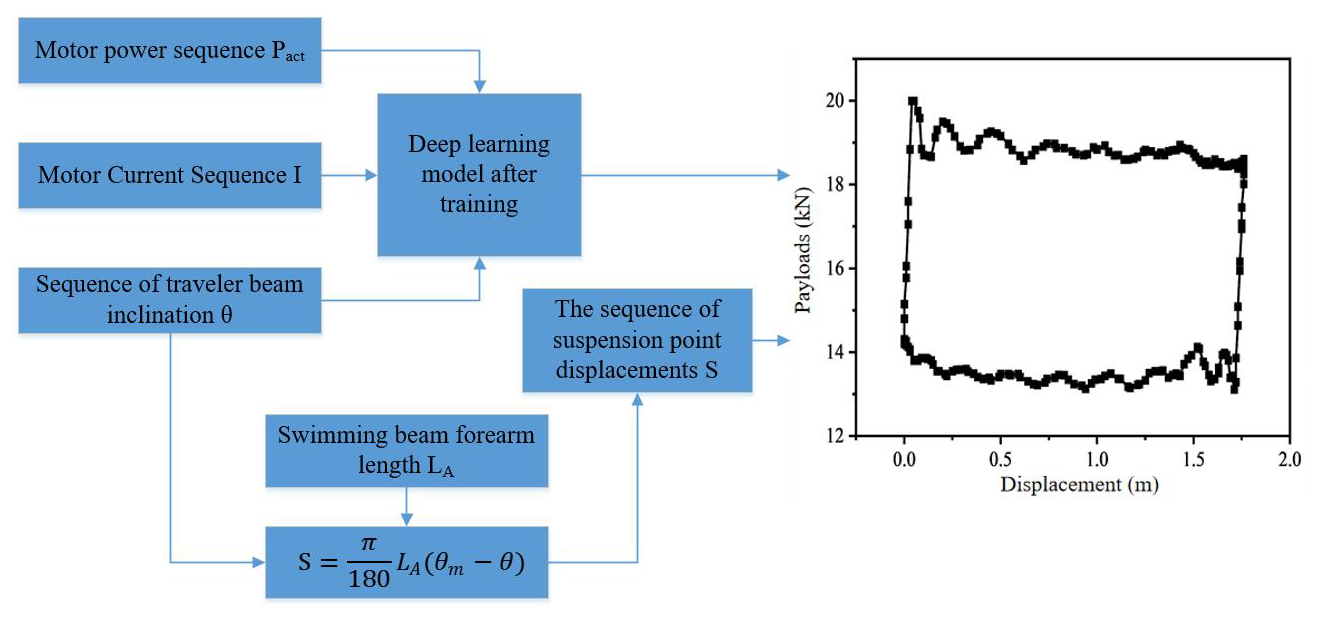
In summary, n measurement points are arranged during the operation of the pumping unit, and the crank angles of the walking beam θ, electric power p_act, and motor current I are recorded as input variables for multi-source data fusion, as illustrated in the corresponding equation. The output of the model is the suspension point load F_p, as shown in Eq. (5). By collecting a sufficient number of datasets, a deep learning model is trained, functioning as a black box that learns the mapping relationship between inputs and outputs during the training phase. As shown in Fig. 1, once the model is trained, the suspension point load can be estimated based on the current cycle's input data. The suspension point displacement is then calculated using the forearm length and the turning angle θ of the walking beam, as described in Eq. (3). Finally, the dynamometer card is constructed based on the estimated suspension point load and displacement.

$$\begin{array}{}\text{(3)}& {\displaystyle }S={\displaystyle \frac{\mathit{\pi }}{\mathrm{180}}}{L}_A\left({\mathit{\theta }}_m-\mathit{\theta }\right)\text{(4)}& {\displaystyle }{\text{TR}}_{\mathrm{in}}={\left[\begin{array}{ccc}{\mathit{\theta }}_{\mathrm{1}}& I_{\mathrm{1}}& P_{\mathrm{act},\mathrm{1}}\\ {\mathit{\theta }}_{\mathrm{2}}& I_{\mathrm{2}}& P_{\mathrm{act},\mathrm{2}}\\ \mathrm{⋮}& \mathrm{⋮}& \mathrm{⋮}\\ {\mathit{\theta }}_n& I_n& P_{\mathrm{act},n}\end{array}\right]}_{n\times \mathrm{3}}\text{(5)}& {\displaystyle }{\text{TR}}_{\mathrm{out}}={\left[\begin{array}{cccc}F{p}_{\mathrm{1}}& F{p}_{\mathrm{2}}& \mathrm{\cdots }& F{p}_n\end{array}\right]}_{\mathrm{1}\times n}^T\end{array}$$

Figure 1 Schematic diagram of the deep-learning-based dynamometer card inversion process.

3 Deep learning inversion model construction for demonstration of power graphs

3.1 CNN-BiGRU Model

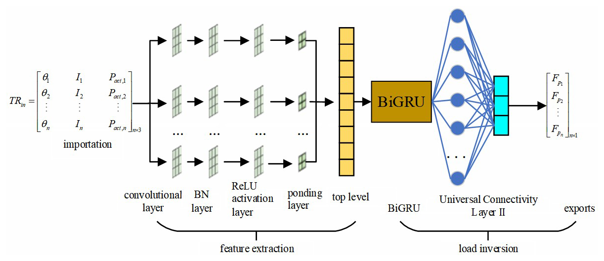
The structure of the CNN-BiGRU model, which integrates a convolutional neural network (CNN) and a bidirectional gated recurrent unit (BiGRU), is illustrated in Fig. 2. The model consists of seven layers: a convolutional layer, a batch normalization (BN) layer, a ReLU activation layer, an average pooling layer, a fully connected layer I, a BiGRU layer, and a fully connected layer II. In this study, the CNN architecture is specifically designed according to the morphological characteristics and scale of dynamometer cards rather than directly adopting a generic deep-image-recognition network. A relatively shallow convolutional structure combined with average pooling is employed to emphasize the global shape features of the load–displacement curves while suppressing local noise, which is beneficial for improving the robustness of the inversion results. Subsequently, the BiGRU layer is introduced to learn the bidirectional temporal dependencies of the extracted features along the time axis. The bidirectional structure enables the model to capture temporal correlations from both past and future states of the sequence, which is consistent with the physical generation process of dynamometer cards involving loading and unloading stages. The learned representations are then passed to the fully connected layers to generate the predicted hanging-point load sequence. By combining task-oriented CNN feature extraction with bidirectional temporal modeling, the proposed CNN-BiGRU framework is able to effectively capture both the spatial morphology and temporal evolution characteristics of dynamometer cards, thereby enhancing inversion accuracy and robustness under complex operating conditions.

Figure 2 Schematic structure of CNN-BiGRU.

The convolutional layer is the core component of the CNN, performing convolution operations on the input data to produce the corresponding feature h_conv for subsequent network learning.

The purpose of the batch normalization (BN) layer is to normalize the output of the convolutional layer so that it has a mean of 0 and a variance of 1, followed by a scaling and shifting process. Batch normalization ensures that the normalized data retain the previously learned features while enhancing network stability, which improves recognition accuracy and accelerates convergence. By applying mini-batch normalization to the features extracted by convolution, the BN layer mitigates the internal covariate shift during training (Ioffe and Szegedy, 2015), thereby speeding up convergence. Additionally, batch normalization reduces the network's dependence on parameter initialization, making the model easier to train. This method also introduces a regularization effect, which helps reduce the risk of overfitting, vanishing gradients, and exploding gradients in the deep network designed in this study. Suppose a batch of input into this layer contains m feature samples h_conv; the main computational steps are as follows.

First, compute the mean μ_f and variance ${\mathit{\sigma }}_f^{\mathrm{2}}$ of the current batch of input samples:

$$\begin{array}{}\text{(6)}& {\displaystyle }{\mathit{\mu }}_f={\displaystyle \frac{\mathrm{1}}{m}}{\sum }_{i=\mathrm{1}}^m{h}_{\mathrm{conv},i},\text{(7)}& {\displaystyle }{\mathit{\sigma }}_f^{\mathrm{2}}={\displaystyle \frac{\mathrm{1}}{m}}{\sum }_{i=\mathrm{1}}^m{\left(h_{\mathrm{conv},i}-{\mathit{\mu }}_f\right)}^{\mathrm{2}}.\end{array}$$

Then normalize the input using the computed mean and variance so that each input feature has zero mean and unit variance. This helps mitigate the problems of vanishing or exploding gradients caused by unstable data distributions during training. The normalization formula is as follows:

$$\begin{array}{}\text{(8)}& \widehat{h_{\mathrm{BN}}}={\displaystyle \frac{h_{\mathrm{conv}}-{\mathit{\mu }}_f}{\sqrt{{\mathit{\sigma }}_f^{\mathrm{2}}+\mathit{\epsilon }}}}.\end{array}$$

In this equation, $\widehat{h_{\mathrm{BN}}}$ denotes the normalized data, and ε is a small constant, typically set to 10⁻⁵, used to prevent division by zero.

To enhance the representational capacity of the network, batch normalization (BN) introduces two trainable parameters: a scaling factor γ and a shifting factor β, which are used to adjust the scale and offset of the normalized data. The transformed output is obtained using the following formula:

$$\begin{array}{}\text{(9)}& h_{\mathrm{BN}}=\mathit{\gamma }\cdot \widehat{h_{\mathrm{BN}}}+\mathit{\beta }.\end{array}$$

ReLU is a nonlinear activation function that is widely used in convolutional neural networks (CNNs) due to its fast convergence and simple gradient computation (Xavier et al., 2011). When a neuron is activated by the ReLU function, inputs of less than zero produce an output of zero, while positive inputs are passed through unchanged. This piecewise linear transformation, known as h_ReLU, enhances the expressive power of the neural network.

The pooling layer is used to compress features, reduce the number of parameters, and retain the most salient characteristics of the output data, thereby accelerating computation. Common pooling methods include max pooling and average pooling. Max pooling selects the maximum value within each pooling region, while average pooling computes the mean of all values within the region. Since all three input features effectively reflect the suspended-point load and because average pooling can smooth feature maps and mitigate over-sensitivity to outlier values, this study adopts average pooling. This approach not only compresses input features efficiently but also preserves global information, ensuring that key characteristics of the input variables are retained. Consequently, it provides a stable input for subsequent feature learning and prediction. The feature map h_ReLU is processed by the average pooling layer, resulting in the output h_pool, as defined in Eq. (10).

$$\begin{array}{}\text{(10)}& y_i^{l+\mathrm{1}}\left(j\right)=\underset{k\in D_j}{max}\left\{x_i^l\left(k\right)\right\}\end{array}$$

In the above equation, $y_i^{l+\mathrm{1}}\left(j\right)$ denotes the element of the ith feature in layer l + 1 after max pooling, $x_i^l\left(k\right)$ represents the element of the ith feature in layer l within the pooling kernel, and D_j denotes the jth pooling region.

As the CNN generates multiple feature maps after feature extraction, a fully connected layer is employed to flatten these maps into a feature vector h_fc, which serves as the input into the BiGRU model. The output of the BiGRU, after sequential processing, is passed through another fully connected layer to produce h_BiGRU. Finally, a regression output layer computes and outputs the suspended-point load sequence TR_out.

3.2 Selection of hyperparameter optimization methods

The CNN-BiGRU model developed in this study is a hybrid architecture. Although increasing the number of nodes and the network depth can enhance the model's learning and fitting capacity, it also significantly increases the number of hyperparameters. These hyperparameters must be set before training, and different combinations can have a substantial impact on model performance, though their effects are often difficult to predict. Evaluating various combinations requires extensive iterative computations, which can be time-consuming.

To improve the learning efficiency and inversion accuracy of the CNN-BiGRU model, the Bayesian optimization (BO) algorithm is employed to determine the optimal set of hyperparameters. Moreover, even when using the same model structure, different hyperparameter combinations can affect model performance across different datasets. As a result, a model trained on a specific dataset may require hyperparameter adjustments for real-world applications in oilfields due to variations in well conditions, pump types, and data characteristics. Therefore, using the Bayesian optimization algorithm not only enables automatic tuning but also facilitates the model's practical deployment in field environments.

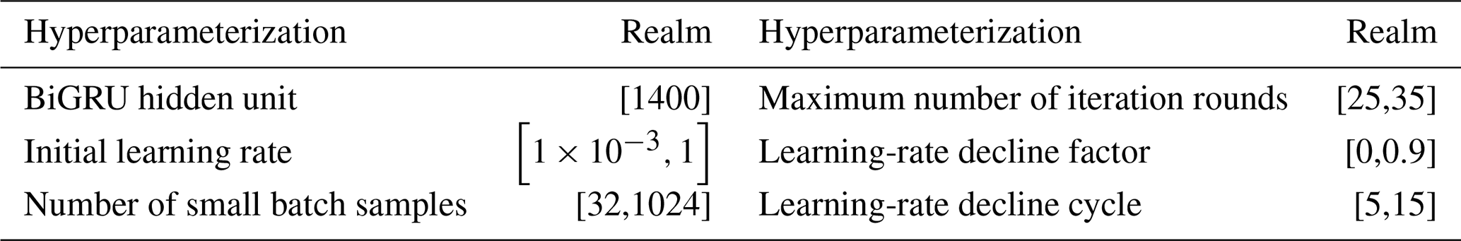
Hyperparameters can generally be categorized into two types: those that define the model architecture and those required by the optimizer. The former are used during both training and inversion, while the latter are only relevant during the training phase. In this model, the hyperparameters selected for optimization include the number of hidden units in the BiGRU, the maximum number of training epochs, the batch size, the initial learning rate, the learning-rate decay factor, and the learning-rate decay period. The number of BiGRU hidden units is an architectural parameter, and optimizing it enhances the model's performance during both training and inversion. Optimizing the maximum number of training epochs, initial learning rate, decay factor, and decay period helps prevent overfitting and improves training accuracy. The batch size determines how training data are fed into the model in mini-batches, thereby accelerating the convergence speed. However, an excessively large batch size may lead to suboptimal local minima, while a very small batch size introduces high randomness and may hinder convergence.

The training error reflects the model's fitting ability on the training data, while the validation error indicates the model's inversion performance. However, a small training error may suggest overfitting, resulting in poor performance on the validation set. By appropriately tuning the initial learning rate, the learning-rate decay factor, and the learning-rate decay period, the model can achieve better training performance. Therefore, to improve the overall performance, the root mean square error (RMSE) of the validation set is selected as the objective function y. The RMSE is calculated as shown in Eq. (11), and the detailed optimization process is illustrated in Fig. 3.

$$\begin{array}{}\text{(11)}& \text{RMSE}=\sqrt{{\displaystyle \frac{\mathrm{1}}{N}}{\sum }_{i=\mathrm{1}}^N{\left(W_i-\widehat{W_i}\right)}^{\mathrm{2}}}\end{array}$$

In this equation, N denotes the number of data points in the validation set, w_i is the actual polished-rod load, and $\widehat{w_i}$ is the predicted polished-rod load.

Figure 3 Hyperparameter-tuning process for Bayesian algorithms.

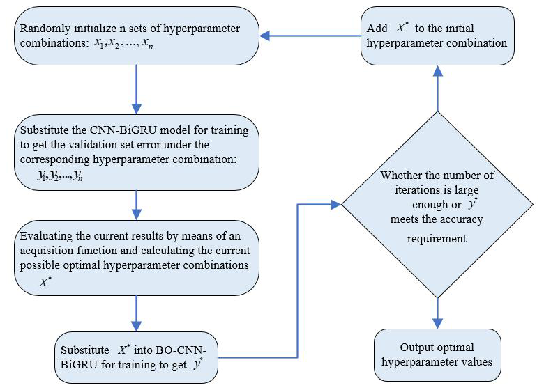
In this study, the Bayesian optimization algorithm employs a Gaussian probabilistic surrogate model to approximate the functional relationship between x and y. First, the search space for each hyperparameter is defined. Then, based on the predefined number of initial points n, n random hyperparameter combinations x_n are generated and used to train the model, yielding the corresponding validation errors y_n. Next, an acquisition function, as defined in Eq. (12), is used to evaluate the current results and to identify the most promising candidate combination x^∗ (Brochu et al., 2010). This candidate is fed into the model to obtain y^∗. The posterior distribution p(y | x,F) of the Gaussian model is then updated. When the posterior distribution closely approximates the true distribution, the optimal set of hyperparameters is considered to be obtained.

$$\begin{array}{}\text{(12)}& E\left(x\right)=\left\{\begin{array}{ll}\left(\mathit{\mu }\left(x\right)-y\left(x^{\ast }\right)\right)\mathrm{\Phi }+\mathit{\sigma }\left(x\right)\mathit{\phi }& \mathit{\sigma }\left(x\right)>\mathrm{0}\\ \mathrm{0}& \mathit{\sigma }\left(x\right)=\mathrm{0}\end{array}\right.\end{array}$$

In this equation, μ(x) denotes the mean of the posterior distribution, and σ(x) represents its variance. y(x^∗) is the objective function value at the current best location. Φ and φ refer to the cumulative distribution function and the probability density function of the standard normal distribution, respectively.

3.3 Workflow of BO-CNN-BiGRU model for dynamometer card inversion

As illustrated in Fig. 4, the workflow of the BO-CNN-BiGRU model, which integrates a convolutional neural network (CNN), bidirectional gated recurrent unit (BiGRU), and Bayesian optimization (BO) algorithm, is presented for the inversion of dynamometer cards. This process is divided into three main components: dataset preparation, model training and parameter tuning, and dynamometer card inversion after training. The detailed procedures for each stage are described as follows.

Figure 4 BO-CNN-BiGRU model schematic power diagram inversion process.

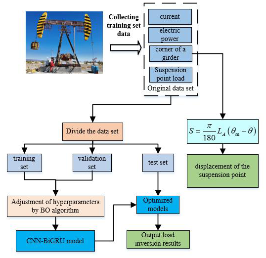
Part I: dataset preparation. Real-time measurements of the polished-rod load (F_P), beam angle (θ), motor current (I), and motor power (p_act) from the pumping unit are collected. After removing cycles with abnormal measurements, the cleaned data form the original dataset for model development.

Since the original input features have different units and magnitudes, normalization is required to convert them into dimensionless data. This process improves the model's adaptability during training by enhancing its ability to capture the intrinsic relationships between variables within the same numerical range. As a result, the model converges more efficiently, and training time is significantly reduced. Normalization is achieved by scaling the data proportionally so that all values are mapped into the range [0,1]. The normalization formula is as follows:

$$\begin{array}{}\text{(13)}& \left\{\begin{array}{l}{x}_{min}=\text{Min}\left(X\right)\\ x_{max}=\text{Max}\left(X\right)\\ f:x⟶y_i=\left(x_i-x_{min}\right)/\left(x_{max}-x_{min}\right)\end{array}.\right.\end{array}$$

In the formula, X represents the original dataset, x_min denotes the minimum value in X, x_max represents the maximum value in X, and y_i is the normalized value.

Part II: model training and parameter tuning. The normalized dataset is divided into training, validation, and test sets. The training set is used for model learning and training, updating the model's weight parameters. The validation set is employed to assess the performance of the model with different parameters at regular intervals during the training process, allowing the model to automatically select and tune parameters to optimize its performance. The test set is used to evaluate the generalization ability of the final optimal model. During the training process, the BO algorithm is utilized for hyperparameter tuning.

Part III: power curve inversion. The trained optimal CNN-BN-BiGRU model is used as the inversion model for the suspended-point load, and its prediction performance is evaluated using the test set. The suspended-point displacement is calculated using the beam angle and the length of the beam forearm, as shown in Eq. (3).

4 Dynamometer card inversion experiment

To validate the effectiveness of the dynamometer card inversion model proposed in this study, it was applied to real oilfield scenarios using actual production data. A comparison model was also established to conduct contrast experiments, demonstrating the advantages of the proposed model.

4.1 Experimental setup

The dynamometer card data were obtained from a specific block in the Xinjiang Oilfield, where real-time monitoring was conducted on pumping units during field operations. Each cycle included 200 uniformly distributed measurement points, capturing data such as polished-rod load F_P, beam angle θ, motor current I, and motor power p_act. After outlier removal, a total of 2500 valid samples were collected. The dataset was divided into training, validation, and testing sets in a ratio of 80 % : 10 % : 10 %.

To evaluate the performance of the proposed BO-CNN-BiGRU model in dynamometer card inversion, a series of comparative experiments were conducted. First, the CNN and BiGRU modules within the BO-CNN-BiGRU model were tested independently. Second, to assess the impact of multi-feature input on inversion accuracy, a comparative experiment was performed using a CNN-BiGRU model with motor power as the sole input, hereinafter referred to as P-CNN-BiGRU. Finally, the proposed model was compared with a traditional BP model that also uses motor power as its only input.

To quantitatively evaluate the inversion accuracy of the model's predicted load, the conformity rate of the calculated load, defined by the dynamic characteristic parameter identification method, is employed as a measure of accuracy. The average matching rate is calculated as shown in Eqs. (14) and (15). The classification criteria for “excellent”, “good”, and “unqualified” levels are defined based on the average conformity rate ranges, as shown in Table 1.

$$\begin{array}{}\text{(14)}& {\displaystyle }{\text{CR}}_i=\left(\mathrm{1}-{\displaystyle \frac{\left|F_{\mathrm{Pi}}^{\mathrm{ref}}-F_{\mathrm{Pi}}\right|}{F_{\mathrm{Pi}}^{\mathrm{ref}}}}\right)\times \mathrm{100}\mathit{\%},i=\mathrm{1},\mathrm{2},\mathrm{\dots },n\text{(15)}& {\displaystyle }{\text{CR}}_{\mathrm{avg}}={\displaystyle \frac{{\sum }_{i=\mathrm{1}}^n{\text{CR}}_i}{n}}\end{array}$$

In the equations, n denotes the number of measured indicator diagram data points within one cycle, $F_{\mathrm{Pi}}^{\mathrm{ref}}$ is the actual value of the suspension load (kN), F_Pi is the calculated value of the suspension load (kN), CR_i denotes the matching rate, and CR_avg denotes the average matching rate.

Table 1 Criteria for defining compliance.

4.2 Experimental results and analysis

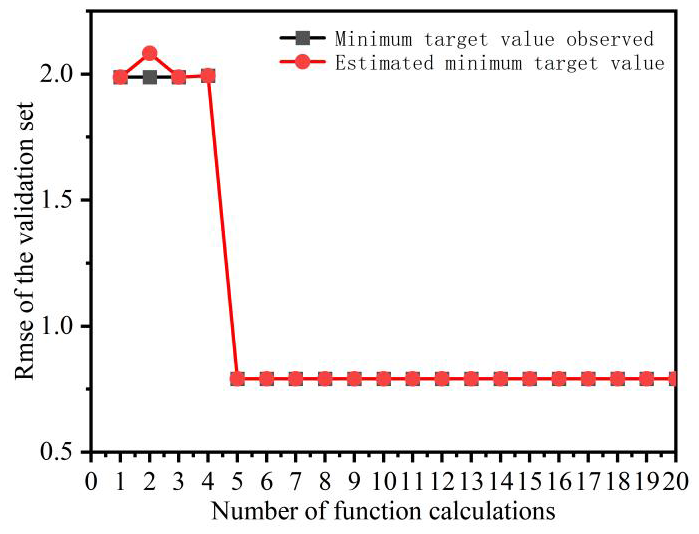
The hyperparameter value ranges for the model are listed in Table 2. The number of initial points for the Bayesian optimization (BO) algorithm was set to 20, with 20 iterations. As shown in Fig. 5, the hyperparameter-tuning process for the CNN-BiGRU model is illustrated. In this process, the “observed value” refers to the actual minimum value recorded during the current iteration, while the “estimated value” refers to the objective value calculated based on the BO model's estimated optimal hyperparameter combination. The model converged after five iterations, i.e., after evaluating 25 sets of hyperparameters. The optimal hyperparameters obtained for the current model are 12 BiGRU hidden units, 27 maximum training epochs, an initial learning rate of 0.0019, a mini-batch size of 34, a learning-rate decay factor of 0.8461, and a decay period of 12. The BO algorithm automatically extracts the optimal values based on observed iteration results, which saves computational resources and time compared to traditional methods. It also enhances the automation and intelligence of the hyperparameter optimization process. This significantly improves the practical applicability of the inversion model, allowing field deployment without requiring domain experts for manual tuning. With only historical data input, the model can be automatically trained to adapt to the specific characteristics of a given oil well.

Table 2 Value range of hyperparameters.

Figure 5 Hyperparameter-tuning iterative process.

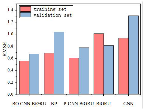
The training performance of the models was evaluated using the root mean square error (RMSE) of the training and validation sets at the end of training. The training results of each model are shown in Fig. 6. As illustrated in the figure, the BO-CNN-BiGRU model achieved lower RMSE values on both the training and validation sets compared to the other models. This indicates that the BO-CNN-BiGRU model attained better fitting performance on the training data. Among the comparison models, the BP and CNN models exhibited relatively high RMSE values on both the training and validation sets, reflecting poor training performance. The P-CNN-BiGRU and BiGRU models demonstrated similar behavior, with RMSE values at a moderate level, slightly higher than those of the BO-CNN-BiGRU model. These results suggest that hybrid models incorporating multi-feature inputs can improve training performance in indicator diagram inversion tasks.

Figure 6 RMSE of the training and validation sets at the end of training for each.

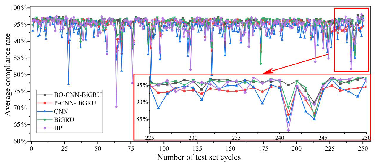
While the model's performance on the training and validation sets reflects its training effectiveness, these results do not fully represent its actual performance. The true indication of the model's real-world applicability lies in its inversion accuracy on the test set, which is not involved in the training process. Therefore, after the model is trained, indicator diagram inversion is conducted using the test set, and the average matching rate across cycles is calculated. The results are shown in Fig. 7. As illustrated in the figure, the BO-CNN-BiGRU model demonstrates stable inversion accuracy throughout the entire test set, with almost no significant fluctuations, indicating reliable performance in indicator diagram inversion tasks. In comparison, the P-CNN-BiGRU model also exhibits a certain level of stability, though this is slightly lower than that of the BO-CNN-BiGRU model. The CNN, BiGRU, and BP models, however, show substantial fluctuations in their matching rates, indicating significantly unstable inversion performance.

Figure 7 Average compliance rate of loads per cycle of the test set.

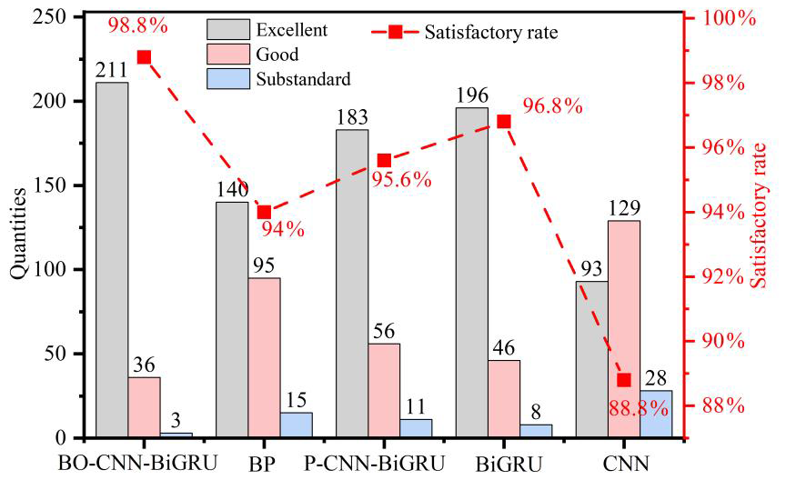
The inversion results of indicator diagrams for each test set were evaluated based on the matching-rate criteria. The evaluation results are shown in Fig. 8. The qualification rates of the five models – BO-CNN-BiGRU, P-CNN-BiGRU, CNN, BiGRU, and BP – were 98.8 %, 95.6 %, 88.8 %, 96.8 %, and 94.0 %, respectively.

Figure 8 Statistical chart of the compliance level of the test set.

Since each indicator diagram contains 200 measurement points per cycle, the average matching rate of a single cycle only reflects the model's accuracy to a limited extent. Figures 9 to 13 present a visual comparison between the inverted and actual indicator diagrams, offering a more intuitive illustration of performance differences among the five models. As shown in the table, the indicator diagrams generated by the BO-CNN-BiGRU model better match the actual diagrams in terms of shape compared with those produced by the other four models.

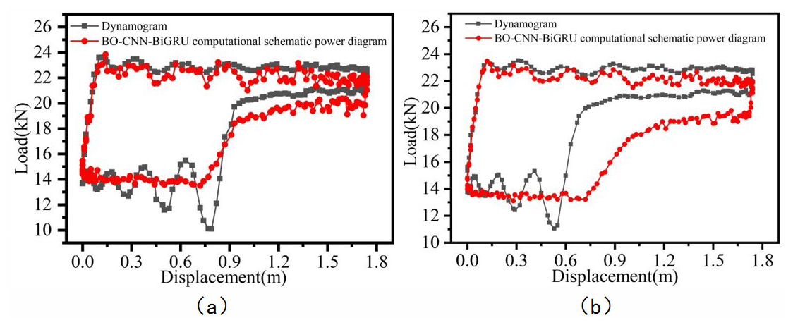
Figure 9 Comparison of inversion results for BO-CNN-BiGRU based on two datasets: (a) dataset 1, (b) dataset 2.

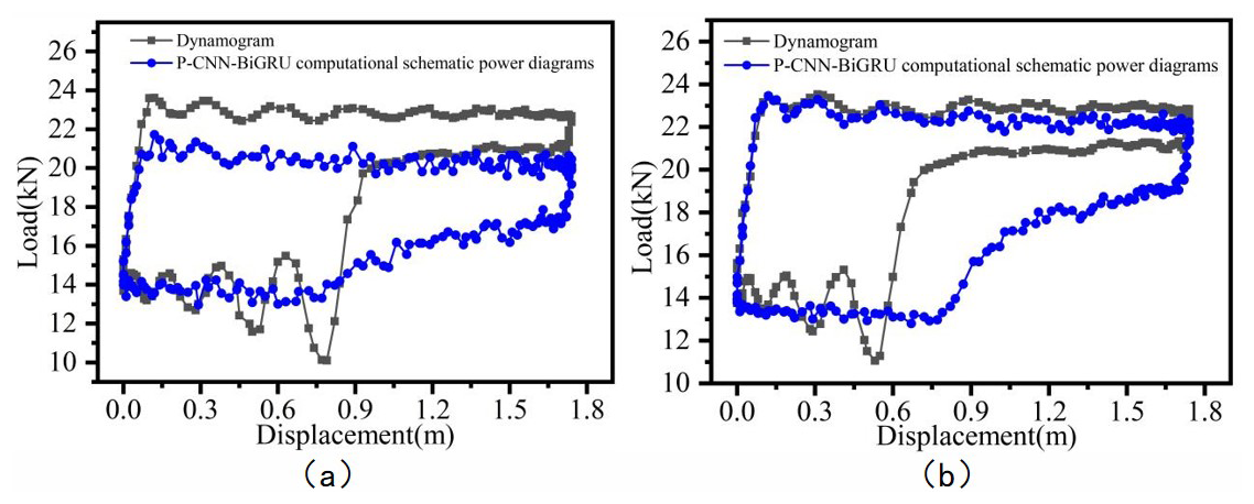
Figure 10 Comparison of inversion results for P-CNN-BiGRU based on two datasets: (a) dataset 1, (b) dataset 2.

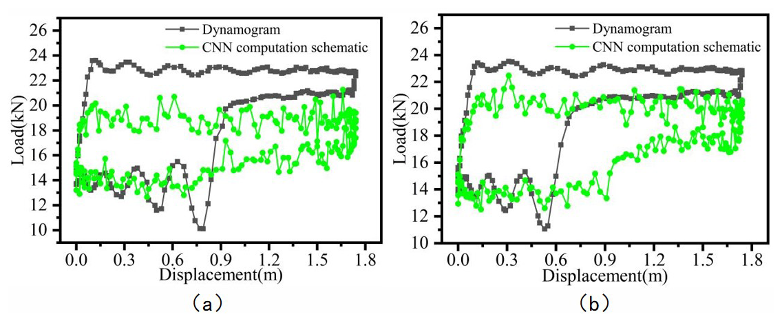
Figure 11 Comparison of inversion results for CNN based on two datasets: (a) dataset 1, (b) dataset 2.

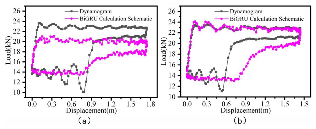
Figure 12 Comparison of inversion results for BiGRU based on two datasets: (a) dataset 1, (b) dataset 2.

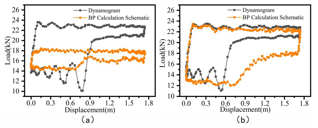
Figure 13 Comparison of inversion results for BP on based on two datasets: (a) dataset 1, (b) dataset 2.

In summary, the effectiveness of the proposed multi-feature hybrid model, BO-CNN-BiGRU, is validated through comparison with four baseline models. By integrating the strengths of convolutional neural networks (CNNs) and bidirectional gated recurrent units (BiGRUs), the BO-CNN-BiGRU model can effectively extract deep features and capture complex temporal dependencies from multi-source data including beam angle (θ), motor current (I), and motor power (P_act), thereby enhancing the accuracy of indicator diagram inversion. The CNN component excels at extracting local patterns from the input data and processing heterogeneous information from different sensors and data sources. Meanwhile, the BiGRU component demonstrates superior capability in modeling temporal dependencies; its bidirectional structure allows it to leverage both past and future information, enabling the model to learn long- and short-term dependencies more effectively and to further improve inversion performance. The integration of these two components improves the model's robustness and accuracy under varying well conditions. By fusing multi-source inputs such as beam angle (θ), motor current (I), and motor power (P_act), the BO-CNN-BiGRU model can more accurately reflect the actual load conditions of the pumping unit, thereby providing reliable indicator diagrams for well monitoring, fault diagnosis, and parameter optimization. In contrast, other models such as BP, CNN, P-CNN-BiGRU, and BiGRU, although capable of inversion to some extent, exhibit limitations in terms of accuracy and stability, making them less practical than the proposed model.

5 Conclusion

In this chapter, an indicator diagram inversion model based on BO-CNN-BiGRU is proposed, which can reconstruct the indicator diagrams of beam pumping units with relatively high accuracy. The model's performance was evaluated using real production data from oilfields, and several baseline models were developed for comparison. The following conclusions are drawn:

• 1.

  Based on an analysis of the pumping unit's mechanical model, output power P_act, motor current I, and beam angle θ were selected as model inputs. As the completeness of the input data increases, the model can better utilize the information contained in each input signal, thereby improving the accuracy of indicator diagram inversion.

• 2.

  The proposed BO-CNN-BiGRU model effectively integrates the deep feature extraction capability of CNN and the temporal feature learning strength of BiGRU. During training, Bayesian optimization is employed to fine-tune the model, which reduces computational cost and training time while enhancing the automation and intelligence of the hyperparameter optimization process. As a result, the model can be deployed across different oil wells without manual tuning – only training data specific to the well are required – thereby improving its practical applicability.

• 3.

  Based on real-case testing results, the BO-CNN-BiGRU model demonstrates superior performance in indicator diagram inversion, outperforming the four baseline models. The qualification rates on the test set for BO-CNN-BiGRU, P-CNN-BiGRU, CNN, BiGRU, and BP were 98.8 %, 95.6 %, 88.8 %, 96.8 %, and 94 %, respectively. Moreover, the proposed model maintains a consistently high match rate of predicted load curves across the entire test set, indicating its ability to accurately capture the complex nonlinear relationships between input variables and load after training.